Visual Representations of Data in Statistics: Categorical and Numerical Variables

Visual Representations of Data

Introduction to Data Visualization

Understanding how data behaves is a fundamental step in statistical analysis. Visualization techniques help us explore the variation and distribution of variables, which can be either categorical or numerical. The choice of graph depends on the type of variable being analyzed.

Visualizing Categorical Variables

Pie Charts and Bar Graphs

Categorical variables represent distinct groups or categories. Two common methods for visualizing categorical data are pie charts and bar graphs.

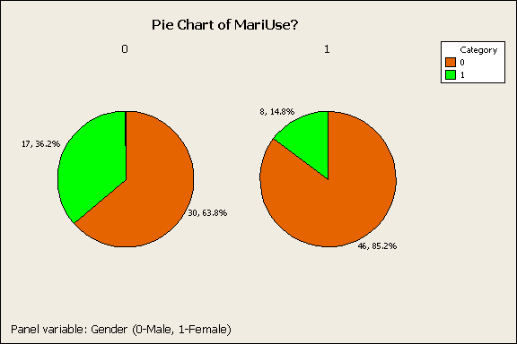
• Pie Charts: Display the proportion of each category as a slice of a circle. Useful for showing relative frequencies.

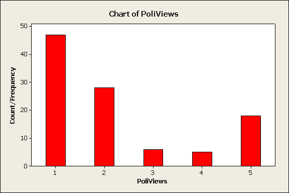
• Bar Graphs: Represent the frequency or count of each category with bars. Useful for comparing sizes across categories.

Example: The breakdown of a sample of first-year university students by gender can be visualized using a pie chart.

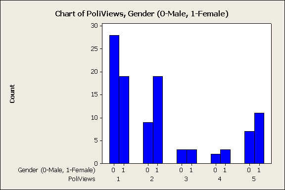
Example: Political views of students can be summarized using bar graphs, both overall and broken down by gender.

Cautions in Graphical Representation

Graphs should not exceed two dimensions for one-dimensional data. Overcomplicating visualizations can lead to misinterpretation.

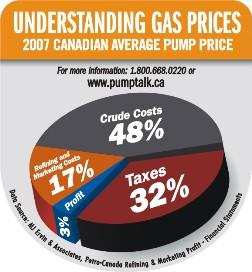
Additional info: The above image illustrates a pie chart used for gas price breakdown, highlighting the importance of clear and appropriate graphical representation.

Visualizing Numerical Variables

Distribution Types

Numerical variables often exhibit certain behaviors, known as their distribution. Common distribution shapes include:

• Symmetrical: Data is evenly distributed around the center.

• Right-skewed: Most data is concentrated on the left, with a tail extending to the right.

• Left-skewed: Most data is concentrated on the right, with a tail extending to the left.

Dotplots

A dotplot is a simple one-dimensional plot where each dot represents a data point. The x-axis shows the values of the numerical variable.

• Example: Survival times (in days) of lung cancer patients can be visualized using a dotplot.

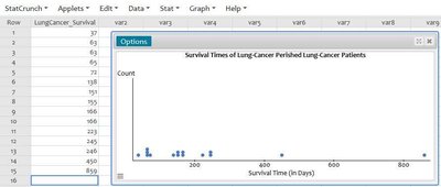
Additional info: Dotplots are useful for visual comparisons between groups or variables.

Histograms

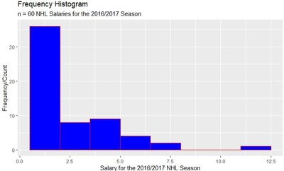
A histogram is a bar graph of a frequency distribution, showing how data points are distributed across intervals (classes).

• Frequency Histogram: Shows the count of data points in each class.

• Relative Frequency Histogram: Shows the proportion of data points in each class.

• Density Histogram: Adjusts for unequal class widths; the area of each bar represents the proportion, and the total area equals 1.

Example: NHL player salaries can be visualized using a frequency histogram.

Constructing Frequency Distributions

To construct a frequency or percentage distribution:

1. Calculate the range: $\text{Range} = \text{Max} - \text{Min}$

2. Determine the number of classes: $k \approx \sqrt{n}$ (where $5 \leq k \leq 15$)

3. Divide the range into $k$ equal intervals: $\text{Width} = \frac{\text{Range}}{k}$

4. Assign each data point to a class and count frequencies.

5. Convert frequencies to percentages for relative frequency distributions.

Frequency Distribution Table Example

The following table summarizes NHL player salaries:

Class	Count/Frequency, $f_i$	Relative Frequency, $p_i = \frac{f_i}{n}$
0.5 < 2.0	36	0.6000
2.0 < 3.5	6	0.1000
3.5 < 5.0	7	0.1167
5.0 < 6.5	8	0.1333
6.5 < 8.0	2	0.0333
8.0 < 9.5	0	0.0000
9.5 < 11.0	0	0.0000
11.0 < 12.5	1	0.0167

Density Histogram Calculation

For unequal class widths, density is calculated as:

• $\text{Density}_{\text{Class }i} = \frac{\text{Relative Frequency}_{\text{Class }i}}{\text{Width}_{\text{Class }i}}$

The area of each bar equals the relative frequency, and the total area is 1.

Empirical Probability from Histograms

Histograms can be used to estimate probabilities. For example, the probability that an NHL player earns less than $3$ million is:

• $P(\text{salary} < 3.0) = (\text{Area Between } 0.5 < 2.0) + (\text{Area Between } 2.0 < 3.0)$

• Using density and width: $P(\text{salary} < 3.0) = (1.5 \times 0.4000) + (1.0 \times 0.0667) = 0.6000 + 0.0667 = 0.6667 \approx 0.67$

Additional info: This approach uses empirical probability based on sample data to estimate proportions in the population.

Summary Exercise: TikTok Influencer Data

Application of Histogram and Density Concepts

Given a sample of TikTok influencers, histograms can be constructed for variables such as average views per post. Key tasks include:

• Creating histograms with specified class boundaries

• Calculating proportions and densities for specific intervals

• Interpreting the shape of the distribution

• Combining classes and recalculating densities

• Estimating counts for extreme values using proportions

Additional info: These exercises reinforce the practical application of visual representation and empirical probability in real-world data analysis.