Week 3 Study Guide: Inference for Counts and Proportions, Probability Distributions, and Hypothesis Testing

Hypothesis Testing

Understanding Hypotheses and Outcomes

Hypothesis testing is a fundamental statistical method used to make inferences about populations based on sample data. The process involves formulating a null hypothesis (H0) and an alternative hypothesis (H1), then using sample data to decide whether to reject H0.

• Null Hypothesis (H0): The default assumption that there is no effect or difference.

• Alternative Hypothesis (H1): The hypothesis that contradicts H0, suggesting an effect or difference exists.

• Type I Error (α): Rejecting H0 when it is actually true.

• Type II Error (β): Failing to reject H0 when it is actually false.

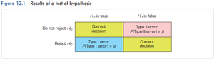
There are four possible outcomes in hypothesis testing:

• Correct decision (do not reject H0 when H0 is true)

• Type I error (reject H0 when H0 is true)

• Type II error (do not reject H0 when H0 is false)

• Correct decision (reject H0 when H0 is false)

P-Value and Statistical Significance

The p-value is a probability, ranging from 0 to 1, that measures the strength of evidence against the null hypothesis. A small p-value (typically < 0.05) indicates strong evidence to reject H0.

• P-value: Probability of obtaining results at least as extreme as the observed results, assuming H0 is true.

• Statistical significance: If p-value < α (significance level), reject H0.

One-Tailed and Two-Tailed Tests

Hypothesis tests can be one-tailed or two-tailed, depending on the research question.

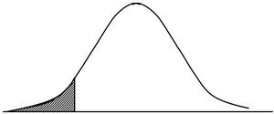
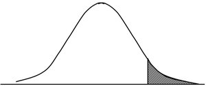
• One-tailed test: Tests for an effect in one direction (e.g., H1: μ > μ0 or μ < μ0).

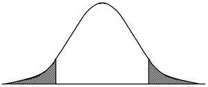
• Two-tailed test: Tests for an effect in either direction (e.g., H1: μ ≠ μ0).

The critical region is split between the tails for two-tailed tests.

Example: One-Tailed Hypothesis Test

Suppose a researcher suspects a coin is biased towards heads. The alternative hypothesis is H1: p > 0.5.

Probability Distributions

Probability Distribution Functions

A probability distribution describes the likelihood of different outcomes for a random variable. Distributions can be visualized as graphs or tables, with the total area under the curve equal to 1.

• X-axis: Possible values of the random variable

• Y-axis: Probabilities or relative frequencies

Probability Mass Function (PMF)

The PMF applies to discrete random variables, assigning a probability to each possible value.

• Formula: $f(x) = P(X = x)$

• Probabilities must be between 0 and 1.

• Example: Rolling a die, the probability of getting a 4 is $\frac{1}{6}$.

Probability Density Function (PDF)

The PDF applies to continuous random variables, describing the probability density for each value.

• Probabilities are found by calculating the area under the curve for a given interval.

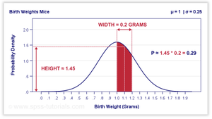
• PDF values can be greater than 1, but the total area under the curve is 1.

Example: Birth Weight of Mice

Birth weights follow a normal distribution with μ = 1 gram and σ = 0.25 grams. The probability that a mouse weighs between 1.0 and 1.2 grams is the area under the curve for that interval.

Cumulative Distribution Function (CDF)

The CDF gives the probability that a random variable is less than or equal to a specified value. It is calculated by summing probabilities from the leftmost value up to the specified value.

Uniform Distribution

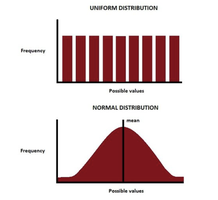
A uniform distribution models scenarios where all outcomes are equally likely.

Normal Distribution

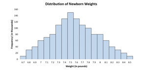
The normal distribution is bell-shaped and symmetric about the mean. It is commonly used for continuous variables such as height, weight, and test scores.

Mathematical Equation

The normal distribution is defined by:

$f(x) = \frac{1}{\sigma \sqrt{2\pi}} e^{-\frac{1}{2} \left( \frac{x-\mu}{\sigma} \right)^2}$

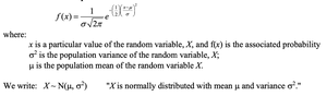
• μ: Mean

• σ: Standard deviation

• π: Pi (≈ 3.14159)

• e: Euler's number (≈ 2.71828)

Properties of the Normal Distribution

• Shape determined by mean (μ) and standard deviation (σ)

• Peak at μ; symmetric about μ

• Mean, median, and mode are equal

• Total area under the curve is 1

Standard Normal Distribution (Z-Distribution)

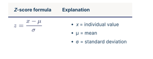
The standard normal distribution has mean 0 and standard deviation 1. Any normal distribution can be converted to the standard normal using the Z-transformation:

$z = \frac{x - \mu}{\sigma}$

Example: SAT Scores

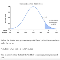
Given a mean SAT score of 1150 and SD of 150, the Z-score for 1380 is:

$z = \frac{1380 - 1150}{150} = 1.53$

From the Z-table, the area to the left of 1.53 is 0.9370. The probability of scores exceeding 1380 is 1 - 0.9370 = 0.063.

Normal Quantile Plots (QQ Plots)

QQ plots are used to visually assess whether data follow a normal distribution. If the points form a straight line, the data are likely normal.

Central Limit Theorem (CLT)

The CLT states that the sampling distribution of the sample mean will be approximately normal if the sample size is large (n ≥ 30), regardless of the population's distribution, provided the population has finite variance.

• Sample size should be sufficiently large (n ≥ 30)

• Samples must be independent and identically distributed

• Population must have finite variance

Binary Data and Binomial Experiments

Binary Data

Binary data consists of two possible outcomes, such as "success" or "failure". Binomial experiments involve repeated independent trials, each with the same probability of success.

Binomial Distribution

The binomial distribution models the number of successes in n independent trials, each with probability p of success.

$f(X = k; n, p) = \binom{n}{k} p^k (1-p)^{n-k}$

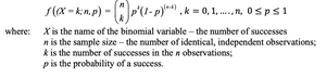
• X: Number of successes

• n: Number of trials

• p: Probability of success

• k: Number of successes

Example: Blood Type O in Children

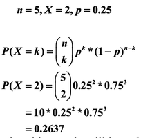
Probability that exactly 2 out of 5 children have blood type O (p = 0.25):

$P(X = 2) = \binom{5}{2} 0.25^2 \times 0.75^3 = 0.2637$

Critical Values and Significance Levels

Critical values are thresholds used to determine whether to reject H0. For binomial tests, critical values may not match the exact significance level due to the discrete nature of the distribution.

Normal Approximation to the Binomial

For large sample sizes, the binomial distribution can be approximated by a normal distribution:

$X \sim N(np, np(1-p))$

• Valid if n > 30, np > 5, and np(1-p) > 5

Example: Proportion of Trees Hosting Epiphytes

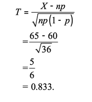
Sample size n = 150, observed successes X = 65, hypothesized proportion p = 0.4.

Normal approximation: $N(60, 36)$

Test statistic:

$T = \frac{X - np}{\sqrt{np(1-p)}} = \frac{65 - 60}{\sqrt{36}} = 0.833$

Critical value for one-tailed test at α = 0.05 is 1.645.

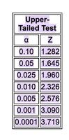
Since T = 0.833 < 1.645, do not reject H0.

Summary Table: Binomial Distribution Example

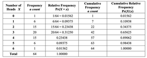
The following table summarizes the distribution of the number of heads in 6 coin tosses:

Number of Heads X	Frequency	Relative Frequency Pr(X=x)	Cumulative Frequency	Cumulative Relative Frequency Pr(X≤x)
0	1	1/64 = 0.01562	1	0.01562
1	6	6/64 = 0.09375	7	0.10938
2	15	15/64 = 0.23438	22	0.34375
3	20	20/64 = 0.31250	42	0.65625
4	15	15/64 = 0.23438	57	0.89062
5	6	6/64 = 0.09375	63	0.98438
6	1	1/64 = 0.01562	64	1.00000
Total	64	1.00000

Conclusion

This study guide covers key concepts in hypothesis testing, probability distributions, and inference for counts and proportions. Understanding these topics is essential for analyzing data and making informed statistical decisions in research.