Z-Scores, Normal Models, and Sampling in Statistics

Z-Scores and Standardization

Definition and Calculation of Z-Scores

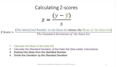
Z-scores are used to standardize data, allowing comparison across different distributions by measuring how many standard deviations an observation is from the mean. The formula for calculating a z-score is:

• Formula: $z = \frac{y - \bar{y}}{s}$

• Steps:

  1. Calculate the mean of the data set.

  2. Calculate the standard deviation of the data set.

  3. Subtract the mean from the identified number.

  4. Divide this deviation by the standard deviation.

• Interpretation: A larger absolute z-score indicates a more uncommon value in the data set. Z-scores can be positive or negative, depending on whether the value is above or below the mean.

Properties of Z-Scores

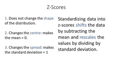
Standardizing data into z-scores does not change the shape of the distribution, but it shifts and rescales the data:

• Shape: Remains unchanged.

• Center: The mean becomes 0.

• Spread: The standard deviation becomes 1.

Density Curves and the Normal Model

Density Curves

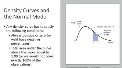
Density curves are smooth curves drawn over histograms to represent the distribution of data. They must satisfy two main conditions:

• Always positive or zero: The curve never dips below the x-axis.

• Total area under the curve: Equals 1, representing 100% of the data.

The Normal Model

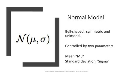
The normal model is a specific type of density curve that is bell-shaped, symmetric, and unimodal. It is defined by two parameters:

• Mean (\mu): Determines the center of the curve.

• Standard deviation (\sigma): Controls the spread of the curve.

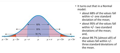
68-95-99.7 Rule

The normal model follows the empirical rule, which describes the proportion of data within certain standard deviations from the mean:

• About 68% of values fall within ±1 standard deviation.

• About 95% fall within ±2 standard deviations.

• About 99.7% fall within ±3 standard deviations.

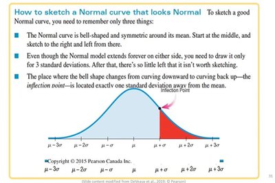
Sketching the Normal Curve

To sketch a normal curve accurately, remember:

• The curve is symmetric and bell-shaped around the mean.

• Draw only up to ±3 standard deviations; beyond this, the curve approaches zero.

• The inflection point occurs one standard deviation from the mean.

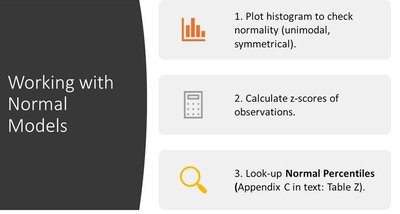
Working with Normal Models

Steps for Analysis

When working with normal models, follow these steps:

• Plot a histogram to check for normality (unimodal, symmetrical).

• Calculate z-scores for observations.

• Look up normal percentiles using statistical tables.

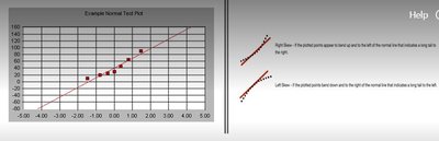
Normal Probability Plots

Normal probability plots are used to check if data follows a normal distribution. If the data points form a straight line, the distribution is approximately normal. Deviations from the line indicate skewness:

• Curving up and to the left: right-skewed (long tail to the right).

• Curving down and to the right: left-skewed (long tail to the left).

Populations, Parameters, and Sampling

Populations and Parameters

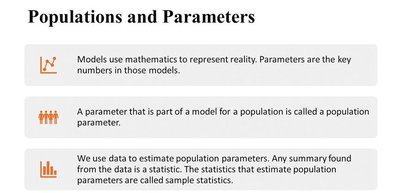
Statistical models use parameters to represent key characteristics of populations. Parameters are estimated using sample statistics:

• Population parameter: A characteristic of the entire population (e.g., mean, standard deviation).

• Sample statistic: A characteristic calculated from a sample, used to estimate the population parameter.

Notation for Statistics and Parameters

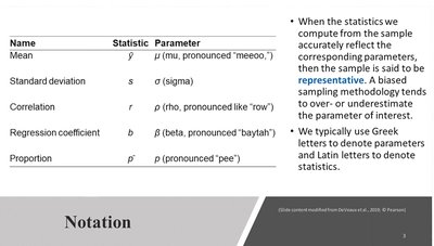
Statistics and parameters are denoted using specific symbols. Greek letters are used for parameters, Latin letters for statistics:

Name	Statistic	Parameter
Mean	\bar{y}	\mu
Standard deviation	s	\sigma
Correlation	r	\rho
Regression coefficient	b	\beta
Proportion	\hat{p}	p

Sampling Methods and Survey Design

Cluster and Multistage Sampling

Cluster sampling involves dividing the population into clusters, then randomly selecting clusters to sample. Multistage sampling combines several methods, often used in large surveys:

• Cluster sampling: Each cluster represents the full population; not all clusters are sampled.

• Multistage sampling: Combines stratified, cluster, and simple random sampling.

From Population to Sample: Sampling Frame and Target Sample

The process of moving from the population to the sample involves several steps, each introducing potential biases:

• The sampling frame is the list from which the sample is drawn.

• The target sample is the group intended to be studied.

• The actual sample consists of respondents.

• Ambiguity in these groups can affect the success and validity of a study.

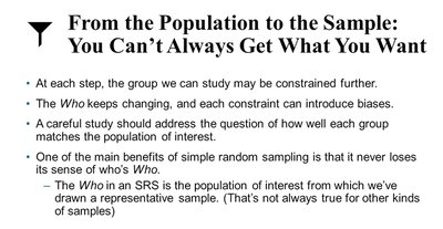
Bias and Constraints in Sampling

Each step in sampling can constrain the group studied and introduce biases. Simple random sampling helps maintain representativeness:

• Constraints may limit which groups can be studied.

• Biases can arise if the sample does not match the population of interest.

• Simple random sampling preserves the sense of 'who's Who' in the population.

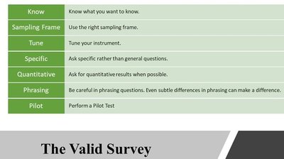
Designing a Valid Survey

To ensure a valid survey, follow these guidelines:

• Know: Define what you want to know.

• Sampling Frame: Use the correct sampling frame.

• Tune: Tune your instrument for data collection.

• Specific: Ask specific questions.

• Quantitative: Prefer quantitative results.

• Phrasing: Phrase questions carefully.

• Pilot: Perform a pilot test.

Common Sampling Mistakes and Biases

Types of Bias

Several biases can affect the validity of survey results:

• Undercoverage: Certain groups are not included in the sample.

• Nonresponse bias: Those who do not respond may differ from those who do.

• Response bias: Survey design influences responses.

• Volunteer bias: Only volunteers are surveyed, which may not represent the population.

• Convenience sampling: Only convenient individuals are sampled, leading to unrepresentative data.

Key Principle: Everyone should have an equal chance of participating in a survey to minimize bias.

Summary Table: Sampling Biases

Bias Type	Description
Undercoverage	Excludes certain groups from the sample
Nonresponse	Differences between respondents and nonrespondents
Response	Survey design influences answers
Volunteer	Only volunteers are surveyed
Convenience	Sample is chosen for convenience

Additional info: These notes cover core concepts from Chapters 5 (The Standard Deviation as a Ruler and the Normal Model) and 10 (Sample Surveys) of a college statistics course, including z-scores, normal models, survey design, and sampling biases.