Aqueous Ionic Equilibria: Buffers and Acid-Base Titrations

Buffer Solutions

Definition, Components, and Properties

Buffer solutions are aqueous systems that resist significant changes in pH when small amounts of strong acid or base are added. They are essential in many chemical and biological processes where maintaining a stable pH is crucial.

• Components: A buffer consists of a weak acid (HA) and its conjugate base (A−), or a weak base (B) and its conjugate acid (BH+).

• Properties: Buffers maintain pH by neutralizing added acids (H+) or bases (OH−).

• Example: Acetic acid (CH3COOH) and sodium acetate (CH3COONa) form a common buffer system.

Understanding Buffer Action

Buffer action is based on the equilibrium between the weak acid and its conjugate base. When acid or base is added, the equilibrium shifts to minimize pH change.

• Acid addition: The conjugate base neutralizes added H+.

• Base addition: The weak acid neutralizes added OH−.

Henderson-Hasselbalch Equation and pH Calculation

The Henderson-Hasselbalch equation relates the pH of a buffer to the concentrations of its acid and base components:

$pH = pK_a + \log \left( \frac{[A^-]}{[HA]} \right)$

• pKa: The negative logarithm of the acid dissociation constant (Ka).

• Application: Used to calculate the pH of buffer solutions and to design buffers with a desired pH.

Preparation of Buffer Solutions

Buffers can be prepared by mixing a weak acid with its salt (conjugate base) or a weak base with its salt (conjugate acid). The ratio of the two components is adjusted to achieve the desired pH.

• Example: To prepare 500 mL of a pH 4.25 buffer using 1.00 M acetic acid and solid sodium acetate (M = 82.034 g/mol, Ka = $1.8 \times 10^{-5}$):

• Calculate the required ratio using the Henderson-Hasselbalch equation.

• Determine the mass of sodium acetate needed and dissolve it in acetic acid, then dilute to the final volume.

Buffer Capacity and Range

Buffer Capacity

Buffer capacity is a measure of a buffer's ability to resist pH changes upon addition of strong acid or base.

• Qualitative: The ability to resist pH change.

• Quantitative: The number of moles of strong acid or base required to change the pH of 1 L of buffer by 1 unit.

• Dependence: Increases with the total concentration of buffer components; maximum when [A−] = [HA].

Buffer Range

The effective pH range of a buffer is typically pKa ± 1. Outside this range, the buffer's ability to resist pH change diminishes.

• Lower limit: $pH = pK_a - 1$

• Upper limit: $pH = pK_a + 1$

• Best resistance: $pH = pK_a$ (when [base]/[acid] ≈ 1)

Calculations Involving Buffers Using the ICE Table

Buffer calculations often use the Initial-Change-Equilibrium (ICE) table to determine equilibrium concentrations and pH.

• Example: For a buffer with 0.30 M acetic acid and 0.20 M sodium acetate (Ka = $1.8 \times 10^{-5}$):

• Set up the equilibrium: $HC_2H_3O_2(aq) + H_2O(l) \rightleftharpoons H_3O^+(aq) + C_2H_3O_2^-(aq)$

• Use the ICE table to solve for [H3O+], then calculate pH.

• Alternatively, use the Henderson-Hasselbalch equation for a quicker calculation.

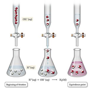
Acid-Base Titrations

Terminology and Concepts

Acid-base titrations are analytical techniques used to determine the concentration of an unknown acid or base by reacting it with a standard solution (titrant).

• Titrant: The solution of known concentration added from a buret.

• Analyte: The solution of unknown concentration in the flask.

• Equivalence point: The point at which stoichiometric amounts of acid and base have reacted.

• Endpoint: The point at which an indicator changes color, signaling the end of the titration.

• Titration error: The difference between the endpoint and the equivalence point.

Acid-Base Titration Curves

A titration curve is a plot of pH versus the volume of titrant added. It provides valuable information about the acid or base being titrated, including the equivalence point and dissociation constants.

• Types of titration curves: Strong acid–strong base, weak acid–strong base, weak base–strong acid, polyprotic acid–strong base.

• Key features: Initial pH, buffer region, equivalence point, and post-equivalence region.

• Applications: Determining unknown concentrations, calculating Ka or Kb, and finding molecular weights.

Strong Acid–Strong Base Titration Example

Consider titrating 50.00 mL of 0.10 M HCl with 0.10 M NaOH. The pH at various stages is calculated as follows:

Volume NaOH Added (mL)	Region	Description	Anticipated pH
0.00	Initial solution	Strong acid solution	Acidic (pH = 1.00)
25.00	Halfway point	Half of strong acid consumed	Acidic (pH = 1.48)
50.00	Equivalence point	All strong acid consumed	Neutral (pH = 7.00)
55.00	Post-equivalence	Excess base solution	Basic (pH = 11.68)

• At equivalence: Only water and neutral salt remain; pH is determined by water autoionization.

• After equivalence: Excess base determines the pH.

Summary Table: Buffer Effectiveness

Condition	pH Expression	Buffer Effectiveness
Lower limit	$pH = pK_a - 1$	Least effective
Upper limit	$pH = pK_a + 1$	Least effective
Best	$pH = pK_a$	Most effective