Aqueous Ionic Equilibrium: Buffers, Titration Curves, and Solubility Equilibria

Chapter 18: Aqueous Ionic Equilibrium

Buffers

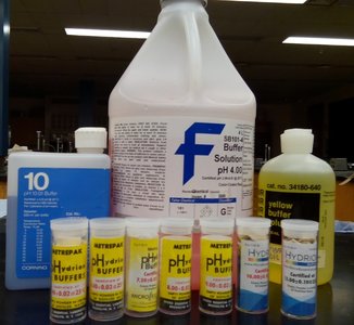
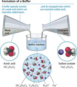
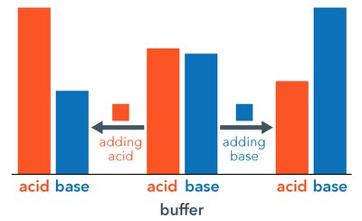
Buffers are solutions that resist changes in pH when small amounts of acid or base are added. They are essential in many chemical and biological systems, including the human body, where blood pH must be tightly regulated. A buffer typically consists of either a weak acid and its conjugate base or a weak base and its conjugate acid.

• Definition: A buffer is a solution that minimizes pH changes upon the addition of an acid or base.

• Composition:

  • Weak acid + its conjugate base (e.g., acetic acid and sodium acetate)

  • Weak base + its conjugate acid (e.g., ammonia and ammonium chloride)

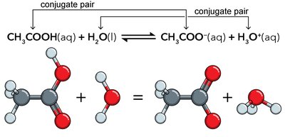
• Example: The acetic acid/sodium acetate buffer system: $\mathrm{CH_3COOH} + \mathrm{CH_3COONa}$

• Biological Application: Blood uses several buffer systems, such as the bicarbonate buffer ($\mathrm{H_2CO_3}/\mathrm{HCO_3^-}$), to maintain pH between 7.35 and 7.45.

How Buffers Work

Buffers function by applying Le Châtelier’s principle to the equilibrium of weak acids or bases. When an acid or base is added, the buffer components react to neutralize the added species, minimizing pH change.

• Reaction with Added Acid: The conjugate base in the buffer reacts with added H+ to form more weak acid.

• Reaction with Added Base: The weak acid in the buffer reacts with added OH- to form more conjugate base and water.

• Example Equilibria:

  • $\mathrm{HA} + \mathrm{OH^-} \rightarrow \mathrm{A^-} + \mathrm{H_2O}$

  • $\mathrm{A^-} + \mathrm{H^+} \rightarrow \mathrm{HA}$

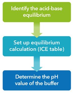
pH Calculations Involving Buffers

To calculate the pH of a buffer, use the equilibrium expression for the weak acid or base, often simplified using the Henderson–Hasselbalch equation. The ICE (Initial, Change, Equilibrium) table is a systematic way to organize concentrations during equilibrium calculations.

• ICE Table: Used to determine equilibrium concentrations for buffer components.

• Henderson–Hasselbalch Equation:

  • $\mathrm{pH} = \mathrm{p}K_a + \log\left(\frac{[\text{base}]}{[\text{acid}]}\right)$

• Example: For a buffer with 0.50 M acetic acid and 0.50 M sodium acetate ($K_a = 1.8 \times 10^{-5}$): $\mathrm{pH} = 4.74$

Buffer Effectiveness: Buffer Range and Buffer Capacity

The effectiveness of a buffer depends on the relative and absolute concentrations of the acid and base components. The buffer capacity is the amount of acid or base a buffer can neutralize before a significant pH change occurs. The buffer range is the pH range over which the buffer is effective, typically $\mathrm{p}K_a \pm 1$.

• Buffer Capacity: Increases with higher concentrations of buffer components.

• Buffer Range: Most effective when $0.1 < \frac{[\text{base}]}{[\text{acid}] } < 10$.

• Choosing a Buffer: Select an acid with a $pK_a$ close to the desired pH.

Titration Curves

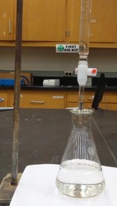
Titration and pH Curves

Titration is a laboratory technique used to determine the concentration of an unknown solution (analyte) by reacting it with a solution of known concentration (titrant). The titration curve is a plot of pH versus the volume of titrant added, and the equivalence point is where stoichiometric amounts of acid and base have reacted.

• Equivalence Point: The point at which the amount of titrant added is stoichiometrically equivalent to the analyte.

• End Point: The point at which the indicator changes color, ideally close to the equivalence point.

• Types of Titrations:

  • Strong acid–strong base

  • Weak acid–strong base

  • Weak base–strong acid

  • Polyprotic acid titrations

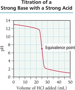
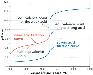
Strong Acid–Base Titrations

In a strong acid–strong base titration, the pH changes rapidly near the equivalence point. Before the equivalence point, the solution contains excess strong acid; after, it contains excess strong base.

• Example Reaction: $\mathrm{HCl} + \mathrm{NaOH} \rightarrow \mathrm{NaCl} + \mathrm{H_2O}$

• Equivalence Point: pH = 7 for strong acid–strong base titrations.

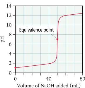
Weak Acid–Strong Base Titrations

When titrating a weak acid with a strong base, the titration curve has a buffer region before the equivalence point. At the half-equivalence point, $\mathrm{pH} = \mathrm{p}K_a$. At the equivalence point, the solution contains the conjugate base, and pH > 7.

• Example: Titration of acetic acid with NaOH.

• Key Regions:

  • Initial pH: determined by weak acid equilibrium

  • Buffer region: mixture of weak acid and conjugate base

  • Equivalence point: only conjugate base present

  • After equivalence: excess strong base

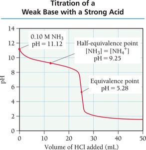
Weak Base–Strong Acid Titrations

In the titration of a weak base with a strong acid, the initial pH is high, and the equivalence point occurs at pH < 7 due to the formation of a weak acid.

• Example: Titration of ammonia with HCl.

• Half-equivalence point: $\mathrm{pOH} = \mathrm{p}K_b$

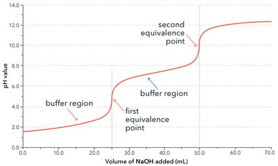
Polyprotic Acid Titrations

Polyprotic acids have more than one ionizable proton, resulting in multiple equivalence points on the titration curve. Each equivalence point corresponds to the neutralization of one proton.

• Example: Titration of sulfurous acid ($\mathrm{H_2SO_3}$) with NaOH shows two equivalence points.

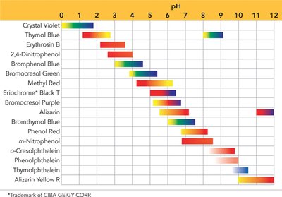
Indicator Selection

Indicators are weak acids or bases that change color at a specific pH range. The best indicator for a titration is one whose color change range includes the equivalence point pH.

• Color Change Range: $\mathrm{pH} = \mathrm{p}K_a \pm 1$

• Example: Phenolphthalein changes from colorless to pink as pH increases from 8.2 to 10.0.

Solubility Equilibria and Solubility Product Constant (Ksp)

Solubility and Ksp

The solubility product constant ($K_{sp}$) is the equilibrium constant for the dissolution of a sparingly soluble ionic compound. It is used to predict whether a precipitate will form and to calculate the solubility of compounds in water.

• General Dissolution Reaction: $\mathrm{MnX_m(s)} \rightleftharpoons n\mathrm{M^{m+}}(aq) + m\mathrm{X^{n-}}(aq)$

• Ksp Expression: $K_{sp} = [\mathrm{M^{m+}}]^n[\mathrm{X^{n-}}]^m$

• Molar Solubility (s): The number of moles of solute that dissolve per liter of solution.

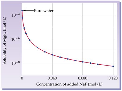
Common Ion Effect on Solubility

The presence of a common ion decreases the solubility of an ionic compound due to Le Châtelier’s principle. Adding a salt that contains a common ion shifts the dissolution equilibrium to the left, reducing solubility.

• Example: Adding NaF to a saturated solution of CaF2 decreases the solubility of CaF2.

Precipitation and Selective Precipitation

Precipitation occurs when the ion product ($Q_{sp}$) exceeds the solubility product constant ($K_{sp}$). Selective precipitation is used to separate ions by adding a reagent that forms an insoluble salt with one ion but not others.

• Precipitation Criteria:

  • $Q_{sp} < K_{sp}$: No precipitate forms (unsaturated)

  • $Q_{sp} = K_{sp}$: Solution is saturated (at equilibrium)

  • $Q_{sp} > K_{sp}$: Precipitate forms (supersaturated)

• Selective Precipitation: Used in qualitative analysis to separate cations based on differences in $K_{sp}$ values.

Complex-Ion Formation Equilibria

Complex ions are formed when a central metal ion binds to one or more ligands. The formation constant ($K_f$) describes the equilibrium for complex ion formation. Complex ion formation can increase the solubility of otherwise insoluble salts.

• Example: $\mathrm{Ag^+} + 2\mathrm{NH_3} \rightleftharpoons \mathrm{Ag(NH_3)_2^+}$

• Effect: Addition of NH3 increases the solubility of AgCl by forming $\mathrm{Ag(NH_3)_2^+}$.

Solubility of Amphoteric Metal Hydroxides

Amphoteric hydroxides can dissolve in both acidic and basic solutions. In acidic solutions, they react with H+ to form soluble species; in basic solutions, they react with excess OH- to form soluble complex ions.

• Examples of Amphoteric Cations: Al3+, Cr3+, Zn2+, Pb2+, Sn2+