 Back
Chapter 18: Aqueous Ionic Equilibrium – Buffers, Titrations, and Solubility
Study Guide - Smart Notes
 Tailored notes based on your materials, expanded with key definitions, examples, and context.
Buffer Solutions and the Common Ion Effect
Definition and Composition of Buffers
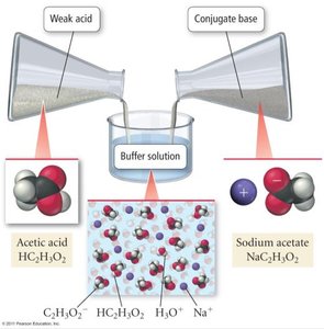
Buffer solutions are mixtures that resist changes in pH when small amounts of acid or base are added. They are composed of a weak acid and its conjugate base, or a weak base and its conjugate acid, typically in approximately equimolar concentrations.
Key Point: Buffers maintain pH stability by neutralizing added acids or bases.
Key Point: The common ion effect occurs when a product ion from one equilibrium reaction inhibits the formation of the same ion in another reaction, shifting equilibrium according to Le Chatelier’s Principle.
Example: A mixture of acetic acid (CH3COOH) and sodium acetate (NaCH3COO) forms a buffer. Acetic acid is the weak acid, and acetate is its conjugate base.
Titration Curves and Buffer Regions
Types of Titration Curves
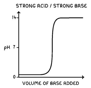
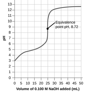
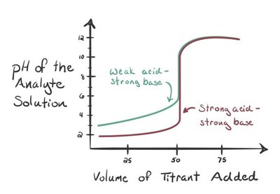
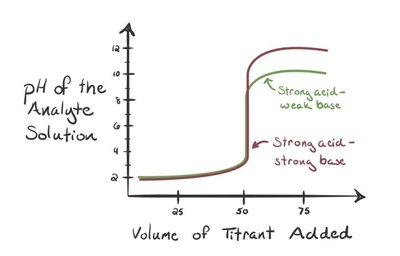
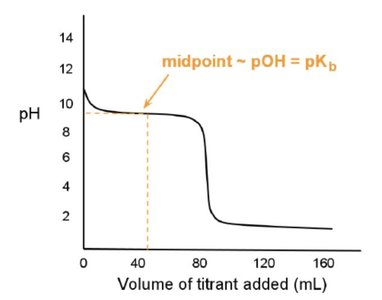
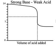
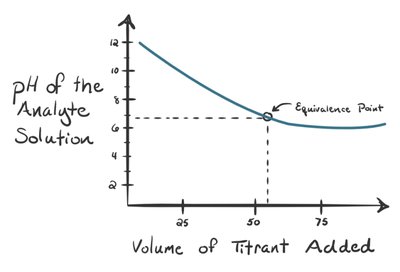
Titration curves plot pH versus the volume of titrant added. The shape of the curve depends on the strength of the acid and base involved.
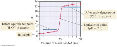
Strong Acid–Strong Base: The equivalence point is at pH = 7, as both reactants are fully dissociated and produce a neutral salt.
Weak Acid–Strong Base: The equivalence point is above pH 7, due to the presence of a basic salt (conjugate base).
Weak Base–Strong Acid: The equivalence point is below pH 7, due to the presence of an acidic salt (conjugate acid).
Buffer Region: Occurs before the equivalence point in weak acid/base titrations, where both acid and conjugate base are present.
Calculating Buffer pH
ICE Table Method
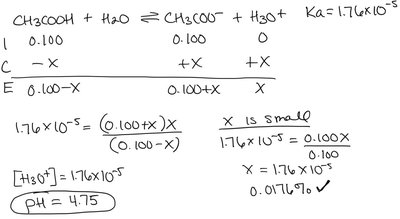
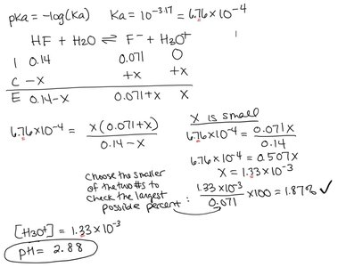
The pH of a buffer can be calculated using an ICE (Initial, Change, Equilibrium) table and the acid dissociation constant (Ka).
Key Point: The ICE table tracks the changes in concentrations of acid, base, and ions during equilibrium.
Example: For 0.100 M CH3COOH and 0.100 M NaCH3COO, use the Ka value and solve for [H3O+].
Henderson-Hasselbalch Equation
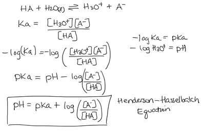
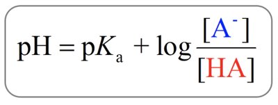
The Henderson-Hasselbalch equation simplifies buffer pH calculations by relating pH to pKa and the ratio of conjugate base to acid concentrations:
Equation:
Key Point: Valid when concentrations are much greater than Ka and the x-is-small approximation holds.
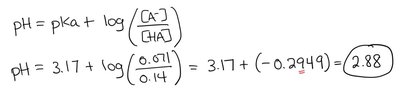
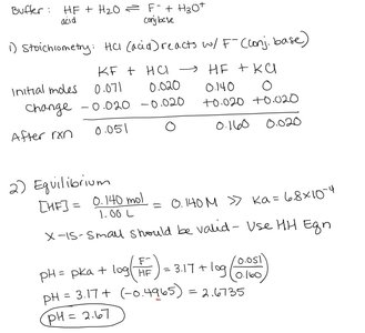
Example: For 0.14 M HF (pKa = 3.17) and 0.071 M KF, pH = 2.88.
Designing Buffers with Specific pH
Choosing Acid/Base Pairs
To create a buffer with a desired pH, select an acid whose pKa is close to the target pH. When [A-] = [HA], pH = pKa.
Key Point: The ratio of conjugate base to acid determines the buffer pH.
Example: To achieve pH 4.25 with formic acid (pKa = 3.75), the ratio [A-]/[HA] should be 3.16.
Buffer Range and Capacity
Buffer Range
The effective range of a buffer is typically within ±1 pH unit of its pKa.
Key Point: Outside this range, the buffer’s ability to resist pH changes diminishes.
Buffer Capacity
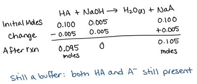
Buffer capacity is the amount of acid or base a buffer can neutralize before its pH changes significantly.
Key Point: Capacity depends on the concentrations of the acid and conjugate base.
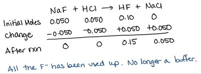
Example: Adding 0.050 mol HCl to a buffer with 0.050 mol NaF destroys the buffer, as all conjugate base is consumed.
Calculating pH Changes in Buffers
Stoichiometry and Equilibrium Calculations
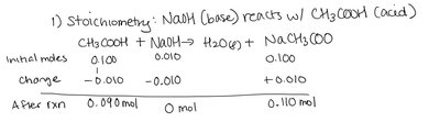
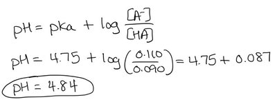
When acid or base is added to a buffer, use stoichiometry to determine new concentrations, then apply the Henderson-Hasselbalch equation if the buffer remains effective.
Key Point: The pH changes slightly, but the buffer resists large shifts.
Example: Adding 0.010 mol NaOH to a buffer of 0.100 mol CH3COOH and 0.100 mol NaCH3COO increases pH from 4.754 to 4.84.
Titration Calculations
Strong Acid/Strong Base Titration
During titration, the pH changes rapidly near the equivalence point. Before equivalence, excess H3O+ is present; after, excess OH- dominates.
Key Point: The equivalence point is at pH = 7 for strong acid/strong base titrations.
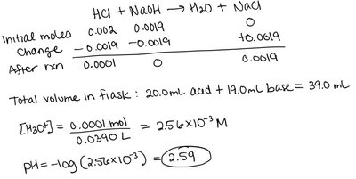
Example: Titrating 20.0 mL of 0.100 M HCl with 19.0 mL of 0.100 M NaOH yields pH = 2.59.

Weak Acid/Strong Base Titration
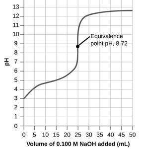
For weak acid titrations, the pH at equivalence is above 7, and the buffer region exists before equivalence. The pH is calculated using ICE tables, stoichiometry, and the Henderson-Hasselbalch equation.
Key Point: At half equivalence, pH = pKa.
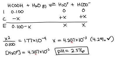
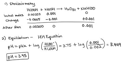
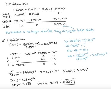
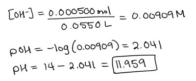
Example: Titrating 25.0 mL of 0.100 M HCOOH with 0.100 M NaOH yields pH = 2.376 initially, pH = 3.45 after 10.00 mL NaOH, pH = 8.225 at equivalence, and pH = 11.959 after excess base.
Comparison of Titration Curves
Different Acid/Base Combinations
The shape and equivalence point of titration curves vary depending on the strengths of acids and bases involved.
Key Point: Strong acid/strong base: equivalence at pH 7; weak acid/strong base: equivalence above pH 7; weak base/strong acid: equivalence below pH 7.
Titration of Polyprotic Acids
Multiple Equivalence Points
Polyprotic acids release protons in steps, each with its own Ka and equivalence point. If Ka values differ significantly, the titration curve shows distinct equivalence points.
Example: H2SO3 titration shows two equivalence points for the two acidic protons.
Solubility and the Solubility Product Constant (Ksp)
Solubility Equilibria
The solubility product constant (Ksp) quantifies the equilibrium between a solid and its dissolved ions in a saturated solution.
Key Point: Small Ksp indicates low solubility.
Example: CaF2(s) → Ca2+(aq) + 2 F-(aq), Ksp = 5.3 × 10⁻⁹.
Common Ion Effect on Solubility
Impact of Added Ions
The presence of a common ion reduces the solubility of a compound by shifting equilibrium toward the solid.
Key Point: CaF2 dissolves less in NaF solution due to the common F- ion.
Ksp and Precipitation
Predicting Precipitation
Precipitation occurs when the ion product (Q) exceeds Ksp. If Q = Ksp, the solution is saturated; if Q < Ksp, unsaturated; if Q > Ksp, precipitation occurs.
Key Point: Use Q and Ksp to predict whether a precipitate will form when solutions are mixed.
Lewis Acids and Bases
Lewis Theory
Lewis acids are electron pair acceptors, while Lewis bases are electron pair donors. This theory explains reactions beyond proton transfer, including complex ion formation.
Key Point: BF3 is a Lewis acid (accepts electrons); NH3 is a Lewis base (donates electrons).
Appendix: Key Equations
Henderson-Hasselbalch Equation:
Solubility Product:
Relationship between pKa and Ka:
