 Back
Chapter 8: Covalent Bonding Theories and Molecular Structure – Study Notes
Study Guide - Smart Notes
 Tailored notes based on your materials, expanded with key definitions, examples, and context.
Chapter 8: Covalent Bonding Theories and Molecular Structure
Molecular Shapes: The VSEPR Model
The Valence Shell Electron Pair Repulsion (VSEPR) model is a theory used to predict the three-dimensional structure of molecules based on the repulsion between electron pairs in the valence shell of the central atom. The arrangement of these electron pairs determines the molecular geometry and bond angles.
Key Point 1: Electron pairs (charge clouds) arrange themselves to minimize repulsion, maximizing their distance from each other.
Key Point 2: Charge clouds include bonds (single, double, triple), lone pairs, and free radicals.
Example: To predict shape, write the Lewis structure, count charge clouds, and assign geometry.
Molecular Shapes: Linear Geometry
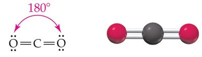
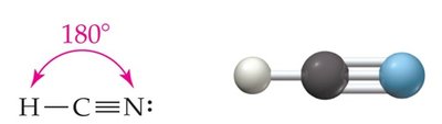
Linear geometry occurs when there are two charge clouds around the central atom. The bond angle is 180°.
Key Point: Any molecule with two charge clouds adopts a linear shape.
Example: CO2 and HCN are linear molecules with 180° bond angles.
Molecular Shapes: Trigonal Planar Geometry
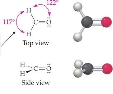
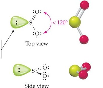
Trigonal planar geometry is observed when there are three charge clouds around the central atom. The ideal bond angle is 120°, but lone pairs can compress angles and change the shape to bent.
Key Point: Three charge clouds result in trigonal planar geometry.
Example: Formaldehyde (CH2O) and sulfur dioxide (SO2) show trigonal planar and bent shapes, respectively.
Molecular Shapes: Tetrahedral Geometry
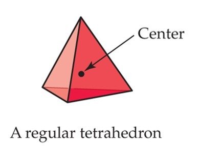
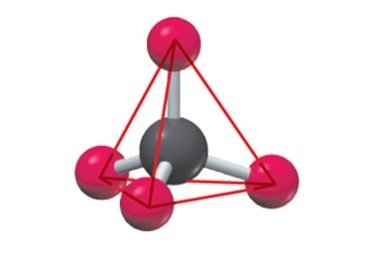
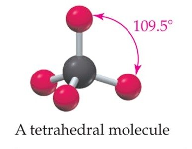
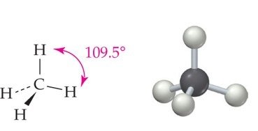
Tetrahedral geometry arises when there are four charge clouds around the central atom. The bond angles are approximately 109.5°.
Key Point: Four charge clouds point to the corners of a tetrahedron.
Example: Methane (CH4) is a classic tetrahedral molecule.
Tetrahedral Geometry with Lone Pairs
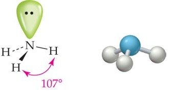
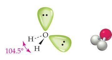
Lone pairs occupy more space than bonding pairs, compressing bond angles. One lone pair yields a trigonal pyramid; two lone pairs yield a bent shape.
Key Point: Lone pairs reduce bond angles and alter molecular shape.
Example: Ammonia (NH3) is trigonal pyramidal; water (H2O) is bent.
Molecular Shapes: Trigonal Bipyramid Geometry
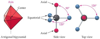
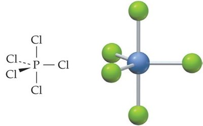
Five charge clouds around a central atom result in trigonal bipyramid geometry, with axial and equatorial positions. Axial positions are 90° from equatorial, and equatorial positions are 120° from each other.
Key Point: Lone pairs prefer equatorial positions due to extra space.
Example: Distortions from lone pairs yield seesaw, T-shaped, or linear shapes.
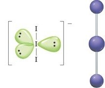
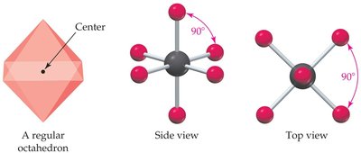
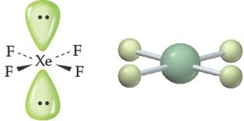
Molecular Shapes: Octahedral Geometry
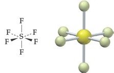
Six charge clouds around a central atom result in octahedral geometry, with all positions equivalent and bond angles of 90°.
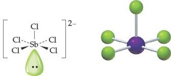
Key Point: Lone pairs can reduce the shape to square pyramid or square planar.
Example: SF6 is octahedral; SbCl62− is square planar.
Valence Bond Theory
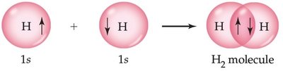
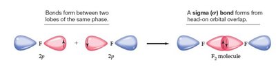
Valence bond theory describes covalent bonds as the overlap of half-filled atomic orbitals, each containing a single electron. The overlap creates a shared electron pair, forming a covalent bond.
Key Point: Covalent bonds form when atomic orbitals overlap and electrons pair.
Example: Sigma (σ) bonds form from head-on overlap; pi (π) bonds from side-by-side overlap.

Hybridization and sp3 Hybrid Orbitals
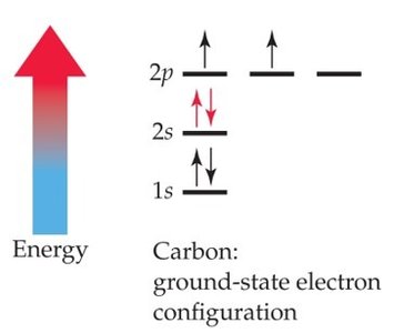
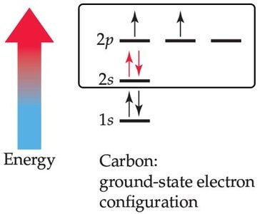
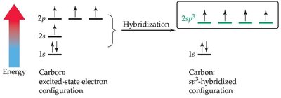
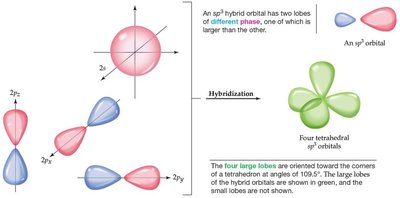
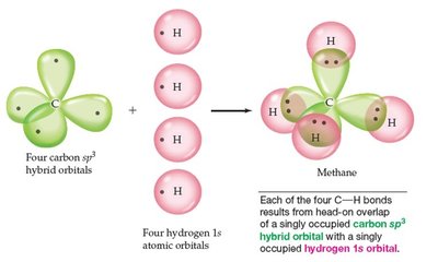
Hybridization explains how atoms like carbon form multiple equivalent bonds. In methane (CH4), carbon's 2s and 2p orbitals mix to form four sp3 hybrid orbitals, each capable of forming a σ bond with hydrogen.
Key Point: Hybrid orbitals are formed by mixing atomic orbitals; the number of hybrid orbitals equals the number mixed.
Example: Four sp3 orbitals point to the corners of a tetrahedron.
Other Hybridization: sp2 and sp Hybrid Orbitals
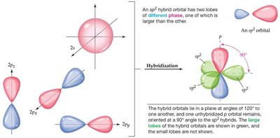
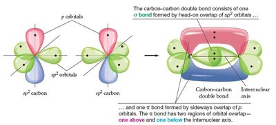
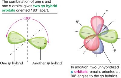
Atoms with three charge clouds use sp2 hybridization (mixing one s and two p orbitals), resulting in three hybrid orbitals in a plane at 120°. Atoms with two charge clouds use sp hybridization (mixing one s and one p orbital), resulting in two linear hybrid orbitals at 180°.
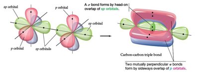
Key Point: Unhybridized p orbitals remain perpendicular to the hybrid orbitals and participate in π bonding.
Example: Double bonds have one σ and one π bond; triple bonds have one σ and two π bonds.
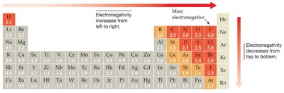
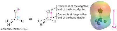
Polar Covalent Bonds and Dipole Moments
Polar covalent bonds arise when atoms with different electronegativities share electrons unequally, creating a dipole moment. The dipole moment (μ) is calculated as:
Formula:
Key Point: The direction of the dipole arrow points from the positive to the negative end.
Example: CH3Cl has a bond dipole due to the electronegativity difference between C and Cl.
Polarity of Molecules
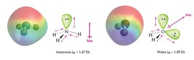
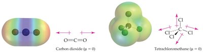
The overall polarity of a molecule depends on the vector sum of individual bond dipoles. If bond dipoles do not cancel, the molecule is polar; if they do, the molecule is nonpolar.
Key Point: NH3 and H2O are polar; CO2 and CCl4 are nonpolar.
Example: The net dipole moment is indicated by the direction and magnitude of the dipole vectors.
Intermolecular Forces (IMFs)
Intermolecular forces are attractions between molecules that influence physical properties such as melting and boiling points. The strength of IMFs varies with the type of force and molecular structure.
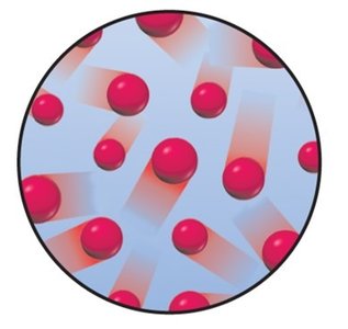
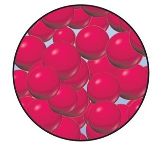
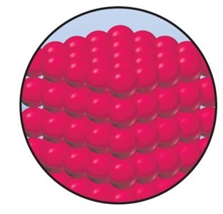
Key Point: Gases have weak IMFs, liquids have moderate IMFs, and solids have strong IMFs.
Example: The state of matter depends on the strength of IMFs.
Types of Intermolecular Forces
IMFs include ion–dipole, dipole–dipole, London dispersion, and hydrogen bonding. The presence or absence of a molecular dipole moment determines the type and strength of these forces.
Key Point: Opposite charges attract, like charges repel.
Example: Hydrogen bonds are much stronger than dipole–dipole or dispersion forces.
London Dispersion Forces
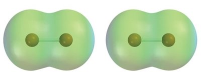
London dispersion forces arise from temporary dipoles induced by the motion of electrons. These forces are present in all molecules and increase with molecular size and polarizability.
Key Point: Larger molecules have stronger dispersion forces and higher boiling points.
Example: Halogens show increasing boiling points with increasing size.
Halogen | mp (K) | bp (K) |
|---|---|---|
F2 | 53.5 | 85.0 |
Cl2 | 171.6 | 239.1 |
Br2 | 265.9 | 331.9 |
I2 | 386.8 | 457.5 |
Dipole–Dipole Forces
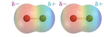
Dipole–dipole forces occur between polar molecules, aligning so that positive and negative ends attract. These forces are stronger than dispersion forces and increase with dipole moment.
Key Point: Preferred orientations maximize attraction and minimize repulsion.
Example: Boiling points increase with dipole moment for molecules of similar size.
Substance | Mol Wt | Dipole Moment (D) | bp (K) |
|---|---|---|---|
CH3CH2CH3 | 44.10 | 0.08 | 231 |
CH3OCH3 | 46.07 | 1.30 | 248 |
CH3CN | 41.05 | 3.93 | 355 |
Hydrogen Bonding
Hydrogen bonding is a strong IMF occurring when hydrogen is bonded to highly electronegative atoms (O, N, F) and interacts with lone pairs on other electronegative atoms. Hydrogen bonds are much stronger than dipole–dipole forces.
Key Point: Hydrogen bonds are responsible for high boiling points and unique properties of water.
Example: Water forms a three-dimensional network of hydrogen bonds, making ice less dense than liquid water.
Ion–Dipole Forces
Ion–dipole forces occur between ions and polar molecules. The strength of these interactions depends on the ion's charge and the dipole moment of the molecule.
Key Point: Ion–dipole forces are stronger than dipole–dipole forces and are important in solutions.
Example: Sodium ions interact strongly with water molecules in solution.
Force | Strength | Characteristics |
|---|---|---|
Ion–dipole | Highly variable (10–70 kJ/mol) | Ions and polar molecules |
Dipole–dipole | Weak (3–4 kJ/mol) | Polar molecules |
London dispersion | Weak (1–10 kJ/mol) | All molecules; depends on size, polarizability |
Hydrogen bond | Moderate (10–40 kJ/mol) | Molecules with O–H, N–H, F–H bonds |
Molecular Orbital Theory (MOT)
MOT describes electrons in molecules using molecular orbitals formed by combining atomic orbitals. The number of molecular orbitals equals the number of atomic orbitals combined. Molecular orbitals can be bonding (lower energy) or antibonding (higher energy).
Key Point: Electrons fill molecular orbitals according to energy and Pauli exclusion principle.
Example: H2 molecule: both electrons occupy the bonding orbital.
Molecular Orbital Theory: Bond Order
Bond order is a measure of bond strength and is calculated as:
Formula:
Key Point: Bond order of 1 indicates a single bond; 0 means no bond forms.
Example: H2: bond order = 1; He2: bond order = 0.
Magnetism and Molecular Orbital Theory
Diamagnetic substances have all electrons paired and are weakly repelled by magnetic fields. Paramagnetic substances have unpaired electrons and are weakly attracted by magnetic fields. O2 is paramagnetic, explained by MOT.
Key Point: Electron-dot structures and valence bond theory cannot explain O2's paramagnetism; MOT can.
Combining Valence Bond and Molecular Orbital Theory
Valence bond theory is used for σ bonds, while MOT explains π bonds and delocalization. For example, in ozone (O3), π electrons are delocalized over all three atoms.
Key Point: MOT provides a more complete picture of bonding and electron distribution.
Chapter Summary
VSEPR: Charge clouds arrange as far apart as possible; lone pairs alter shape and compress bond angles.
Valence bond theory: Bonds form by overlap of half-filled orbitals; hybrid orbitals (sp, sp2, sp3) explain geometry.
Multiple bonds: Contain one σ bond plus one or two π bonds.
Polarity: A molecule is polar if its bond dipoles do not cancel.
Intermolecular forces: Ion–dipole, dipole–dipole, London dispersion, hydrogen bonds.
MOT: Explains bond order and magnetism (e.g., O2 paramagnetism).
