Chemical Equilibrium: Principles, Expressions, and Applications

Unit 7: Chemical Equilibrium

Introduction to Equilibrium

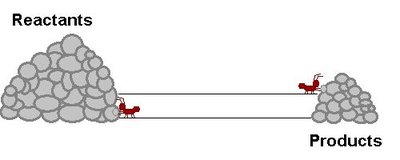
Chemical equilibrium is a fundamental concept in chemistry, describing a state in which the rates of the forward and reverse reactions are equal, resulting in constant concentrations of reactants and products. Many chemical and physical processes are reversible, and equilibrium is established when these processes occur simultaneously at equal rates.

• Dynamic Equilibrium: At equilibrium, reactants and products are present in constant amounts, but the reactions continue to occur in both directions.

• Observable Processes: Examples include phase changes (evaporation/condensation), dissolution/precipitation, acid-base reactions, and redox reactions.

• Graphical Representation: Equilibrium can be visualized using graphs of concentration or rate versus time.

• Criteria for Reversibility: Both forward and reverse rates must be significant and observable.

Example: The decomposition of dinitrogen tetroxide: N2O4(g) ⇌ 2NO2(g)

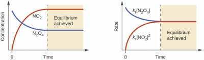
Additional info: The graphical representation shows how concentrations and reaction rates stabilize once equilibrium is reached.

Direction of Reversible Reactions

The direction in which a reversible reaction proceeds depends on the relative rates of the forward and reverse reactions. Initially, the forward rate is greater, leading to an increase in product concentration. As the reaction progresses, the reverse rate increases until both rates are equal and equilibrium is established.

• Forward vs. Reverse Rate: If the forward rate > reverse rate, products are formed. If the reverse rate > forward rate, reactants are formed.

• Equilibrium State: No net change in concentrations; rates are equal.

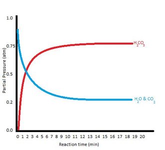
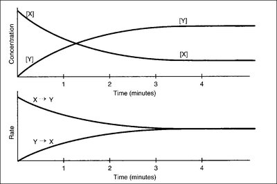
Additional info: These graphs illustrate how equilibrium is achieved as concentrations and rates stabilize.

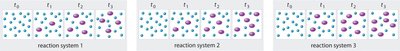
Particulate Representations of Equilibrium

Particulate diagrams are used to visually represent the relative numbers of reactant and product particles before and at equilibrium. These models help students understand the dynamic nature of equilibrium at the molecular level.

• Interpretation: At equilibrium, the ratio of reactant to product particles remains constant.

• Application: Useful for predicting shifts in equilibrium and understanding the effect of changes in conditions.

Equilibrium Expressions: Reaction Quotient (Q) and Equilibrium Constant (K)

The equilibrium constant (K) describes the ratio of product to reactant concentrations at equilibrium. The reaction quotient (Q) is calculated at any point in the reaction and is used to predict the direction in which the reaction will proceed to reach equilibrium.

• For a general reaction: aA + bB ⇌ cC + dD

• Equilibrium Expression:

$K_c = \frac{[C]^c[D]^d}{[A]^a[B]^b}$

$K_p = \frac{(P_C)^c(P_D)^d}{(P_A)^a(P_B)^b}$

• Exclusion: Pure solids and liquids are not included in the equilibrium expression.

• Qc and Qp: Qc uses concentrations (M), Qp uses partial pressures (atm).

Calculating the Equilibrium Constant

Equilibrium constants can be determined from experimental measurements of concentrations or partial pressures at equilibrium. Calculations may involve straightforward algebra or the use of ICE (Initial, Change, Equilibrium) tables.

• Example: For the reaction 2HI(g) ⇌ H2(g) + I2(g), if [HI] = 3.53 × 10-3 M and [H2] = 4.79 × 10-4 M at equilibrium:

$K_c = \frac{[H_2][I_2]}{[HI]^2}$

Magnitude of the Equilibrium Constant

The value of K indicates the extent to which a reaction proceeds:

• Large K: Reaction favors products; proceeds nearly to completion.

• Small K: Reaction favors reactants; little product is formed.

• K ≈ 1: Significant amounts of both reactants and products are present.

Properties of the Equilibrium Constant

The equilibrium constant changes in predictable ways when the chemical equation is manipulated:

• Reversing the reaction: K is inverted.

• Multiplying coefficients: K is raised to the corresponding power.

• Adding reactions: K values are multiplied.

Calculating Equilibrium Concentrations

Given initial conditions and the equilibrium constant, equilibrium concentrations can be calculated using algebraic methods or ICE tables.

• ICE Table: Organizes initial concentrations, changes, and equilibrium concentrations.

• Application: Useful for complex reactions and when initial and equilibrium values are known.

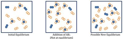
Le Châtelier’s Principle

Le Châtelier’s principle states that a system at equilibrium will respond to external stresses by shifting in a direction that relieves the stress and establishes a new equilibrium.

• Types of Stress: Addition/removal of reactant or product, changes in temperature, pressure, or volume, dilution, and addition of a catalyst.

• Effect of Stress: The system shifts to increase or decrease the concentration of products or reactants as needed.

• Example: Adding more NH3 to N2(g) + 3H2(g) ⇌ 2NH3(g) shifts the equilibrium to the left.

Reaction Quotient and Le Châtelier’s Principle

When a system is disturbed, Q differs from K, and the system shifts to restore equilibrium:

• If Q < K: Reaction shifts right (toward products).

• If Q > K: Reaction shifts left (toward reactants).

• If Q = K: System is at equilibrium; no shift occurs.

Solubility Equilibria and the Common-Ion Effect

The dissolution of salts is a reversible process described by the solubility product constant (Ksp). The solubility of a salt can be calculated from Ksp, and the presence of a common ion reduces solubility (common-ion effect).

• Ksp Expression: For AgCl(s) ⇌ Ag+(aq) + Cl-(aq): $K_{sp} = [Ag^+][Cl^-]$

• Solubility Calculation: If Ksp = 1.8 × 10-10, then $x^2 = 1.8 \times 10^{-10}$; $x = 1.3 \times 10^{-5}$ M

• Common-Ion Effect: Adding NaCl increases [Cl-], reducing [Ag+] and the solubility of AgCl.

Additional info: The common-ion effect can be assessed qualitatively using Le Châtelier’s principle and quantitatively using Ksp.