Solutions and Their Properties (General Chemistry II, Ch. 13 Study Notes)

Solutions and Their Properties

Introduction to Solutions

Solutions are homogeneous mixtures composed of two or more substances. The study of solutions is fundamental in chemistry, as it relates to solubility, concentration, and the physical properties of mixtures. This chapter explores the energetics, structure, and behavior of solutions, with a focus on aqueous systems.

Solubility and Intermolecular Forces

Predicting Solubility

• Solubility is the ability of a solute to dissolve in a solvent to form a homogeneous mixture.

• "Like dissolves like": Polar solutes dissolve in polar solvents, and nonpolar solutes dissolve in nonpolar solvents.

• Key factors: Intermolecular forces (IMFs), molecular polarity, and the structure of solute and solvent molecules.

• Types of solids: Covalent, ionic, atomic/network solids.

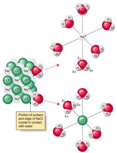
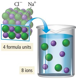
Example: Water (a polar solvent) dissolves ionic compounds like NaCl due to strong ion-dipole interactions.

Energetics of Solution Formation

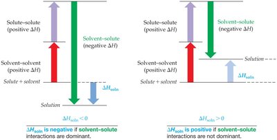
• Enthalpy of solution (ΔHsolution): The overall energy change when a solution forms.

• Steps in solution formation:

  • Breaking solute-solute IMFs (endothermic, ΔH > 0)

  • Breaking solvent-solvent IMFs (endothermic, ΔH > 0)

  • Forming solute-solvent IMFs (exothermic, ΔH < 0)

• ΔHsolution = ΔHsolute-solute + ΔHsolvent-solvent + ΔHsolute-solvent

• Solutions form when the energy released in forming solute-solvent interactions compensates for the energy required to separate solute and solvent particles.

Solvation and Entropy

• Solvation: The process of surrounding solute particles with solvent molecules.

• Entropy (ΔS): A measure of molecular randomness or disorder. Dissolution increases entropy (ΔS > 0).

• Spontaneity of solution formation is determined by Gibbs Free Energy (ΔG):

$\Delta G_{solution} = \Delta H_{solution} - T\Delta S_{solution}$

• A process is spontaneous if ΔG < 0.

Concentration Units

Common Concentration Units

• Mass percent (%): $\frac{\text{mass of solute}}{\text{mass of solution}} \times 100$

• Mole fraction (χ): $\chi_A = \frac{n_A}{n_A + n_B + \ldots}$

• Molarity (M): $M = \frac{\text{moles of solute}}{\text{liters of solution}}$

• Molality (m): $m = \frac{\text{moles of solute}}{\text{kg of solvent}}$

Example: Calculate the molality of a solution containing 1.00 g ethanol in 100.0 g water: $m = 0.217$ m.

Types of Mixtures: Solutions, Colloids, and Suspensions

Classification of Mixtures

• Solution: Homogeneous mixture, particle size 0.1–2 nm (e.g., saltwater).

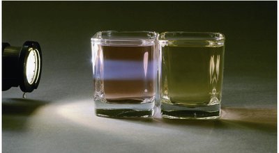
• Colloid: Heterogeneous mixture, particle size 2–1000 nm, exhibits the Tyndall effect (e.g., milk).

• Suspension: Heterogeneous mixture, particle size >1 μm, particles settle out (e.g., muddy water).

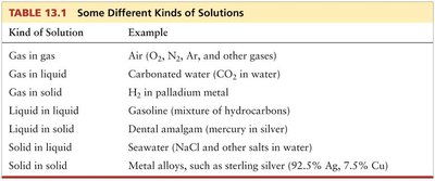
Types of Solutions

Kind of Solution	Example
Gas in gas	Air (O2, N2, Ar, etc.)
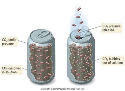
Gas in liquid	Carbonated water (CO2 in water)
Gas in solid	H2 in palladium metal
Liquid in liquid	Gasoline (mixture of hydrocarbons)
Liquid in solid	Dental amalgam (mercury in silver)
Solid in liquid	Seawater (NaCl and other salts in water)
Solid in solid	Metal alloys (e.g., sterling silver)

Solubility Trends

Temperature and Pressure Effects

• Solubility of solids generally increases with temperature.

• Solubility of gases decreases with increasing temperature but increases with pressure (Henry's Law).

Henry's Law: $C_{gas} = k_H P_{gas}$

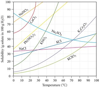
Solubility Curves

• Solubility curves show how much solute dissolves in 100 g of water at various temperatures.

• Used to determine if a solution is saturated, unsaturated, or supersaturated at a given temperature.

Colligative Properties

Definition and Types

• Colligative properties depend on the number of solute particles, not their identity.

• Key colligative properties:

  • Vapor pressure lowering

  • Boiling point elevation

  • Freezing point depression

  • Osmotic pressure

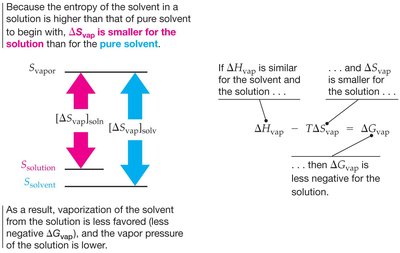
Vapor Pressure Lowering and Raoult's Law

• Adding a non-volatile solute lowers the vapor pressure of the solvent.

• Raoult's Law: $P_{solution} = \chi_{solvent} P^\circ_{solvent}$

Boiling Point Elevation and Freezing Point Depression

• Boiling point elevation: $\Delta T_b = m \times i \times K_b$

• Freezing point depression: $\Delta T_f = m \times i \times K_f$

• Where m is molality, i is the van't Hoff factor, and K_b, K_f are solvent-specific constants.

Example: Calculate the freezing point of a 0.89 m CaCl2 solution (i = 3): $\Delta T_f = (0.89)(3)(1.86) = 4.97^\circ C$ New freezing point = $0.0^\circ C - 4.97^\circ C = -5.0^\circ C$

Osmotic Pressure

• Osmotic pressure ($\pi$) is the pressure required to stop osmosis.

• Calculated by: $\pi = iMRT$

• Where M is molarity, R is the gas constant, T is temperature in Kelvin, and i is the van't Hoff factor.

Van't Hoff Factor and Ion Pairing

• The van't Hoff factor (i) is the number of particles a solute produces in solution.

• For non-electrolytes, i = 1; for ionic compounds, i equals the number of ions formed.

• Ion pairing can cause deviations from the ideal value of i.

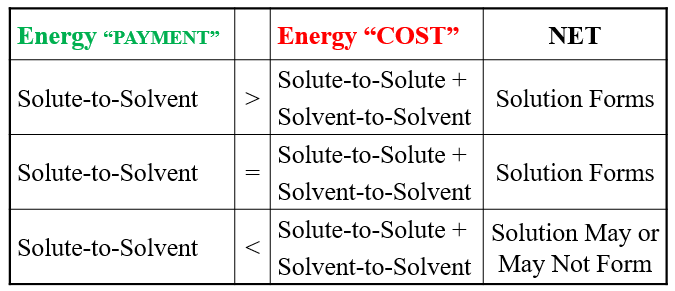
Summary Table: Energy Considerations in Solution Formation

Energy "PAYMENT"	Energy "COST"	NET
Solute-to-Solvent >	Solute-to-Solute + Solvent-to-Solvent	Solution Forms
Solute-to-Solvent =	Solute-to-Solute + Solvent-to-Solvent	Solution Forms
Solute-to-Solvent <	Solute-to-Solute + Solvent-to-Solvent	Solution May or May Not Form

Practice Problems and Applications

• Calculate concentrations using different units (molarity, molality, mole fraction, mass percent).

• Apply colligative property equations to determine boiling point elevation, freezing point depression, and osmotic pressure.

• Interpret solubility curves and predict solution behavior under varying conditions.

Key Equations

• $\Delta H_{solution} = \Delta H_{solute-solute} + \Delta H_{solvent-solvent} + \Delta H_{solute-solvent}$

• $\Delta G_{solution} = \Delta H_{solution} - T\Delta S_{solution}$

• $P_{solution} = \chi_{solvent} P^\circ_{solvent}$

• $\Delta T_b = m \times i \times K_b$

• $\Delta T_f = m \times i \times K_f$

• $\pi = iMRT$

• $C_{gas} = k_H P_{gas}$

Additional info: For cumulative problems, use logical assumptions (e.g., 100 g solution for mass %, 1 L for molarity, 1 kg solvent for molality) to simplify calculations.