Ch. 9 - Differential Equations
Briggs - Calculus: Early Transcendentals 3rd Edition
Briggs3rd EditionCalculus: Early TranscendentalsISBN: 9780136847243Non è quello che usi tu?Cambia libro di testo
Capitolo 9, Problema 9.5.15

15–16. {Use of Tech} Solving logistic equations Write a logistic equation with the following parameter values. Then solve the initial value problem and graph the solution. Let r be the natural growth rate, K the carrying capacity, and P₀ the initial population.


r=0.2, K=300, P₀=50

Guida verificata passo dopo passo
1
Start by writing the general form of the logistic differential equation: \[\frac{dP}{dt} = rP\left(1 - \frac{P}{K}\right)\] where \(P(t)\) is the population at time \(t\), \(r\) is the natural growth rate, and \(K\) is the carrying capacity.
Substitute the given parameter values into the logistic equation: \[\frac{dP}{dt} = 0.2P\left(1 - \frac{P}{300}\right)\].
Set up the initial value problem (IVP) by including the initial condition: \[P(0) = 50\].
To solve the IVP, separate variables and integrate: rewrite the equation as \[\frac{dP}{P(1 - P/300)} = 0.2\,dt\] and then perform partial fraction decomposition on the left side before integrating both sides.
After integrating, solve for \(P(t)\) explicitly in terms of \(t\) and the constants, then use the initial condition \(P(0) = 50\) to find the constant of integration. This will give you the logistic growth function describing the population over time.

Risposta video verificata per un problema simile:

Questa soluzione video è stata consigliata dai nostri tutor come utile per risolvere questo problema.
Durata del video:
8m

Concetti chiave

Ecco i concetti essenziali che devi comprendere per rispondere correttamente alla domanda.

Logistic Growth Model

The logistic growth model describes population growth that starts exponentially but slows as the population approaches a maximum limit called the carrying capacity (K). It is represented by the differential equation dP/dt = rP(1 - P/K), where r is the natural growth rate and P is the population at time t.
Video consigliato:
09:29
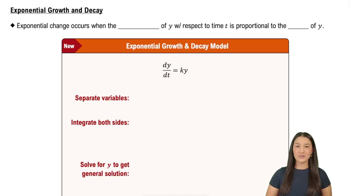
Exponential Growth & Decay

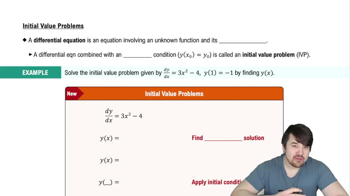
Solving Initial Value Problems (IVPs)

An initial value problem involves solving a differential equation with a given initial condition, such as P(0) = P₀. Solving the logistic equation IVP means finding a function P(t) that satisfies both the logistic differential equation and the initial population value.
Video consigliato:
Percorso guidato
05:03
Initial Value Problems

Graphing Solutions of Differential Equations

Graphing the solution to a logistic equation shows how the population changes over time, typically starting at P₀, growing rapidly, and leveling off near the carrying capacity K. This visual helps interpret the behavior and stability of the population model.
Video consigliato:
04:00
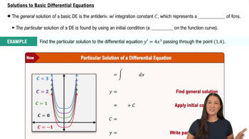
Solutions to Basic Differential Equations