Ch. 5 - Integration

Briggs - Calculus: Early Transcendentals 3rd Edition

Briggs3rd EditionCalculus: Early TranscendentalsISBN: 9780136847243당신이 사용하는 게 아니라요?교과서 변경

Briggs 3rd Edition

Ch. 5 - Integration

문제 5.4.53a

5장, 문제 5.4.53a

Average value with a parameter Consider the function ƒ(𝓍) = a𝓍 (1―𝓍) on the interval [0, 1], where a is a positive real number.
(a) Find the average value of ƒ as a function of a .

검증된 단계별 안내

Step 1: Recall the formula for the average value of a function ƒ(𝓍) on the interval [a, b], which is given by:

\frac{1}{(b - a)} \int f_{x} d x

. In this case, the interval is [0, 1] and the function is ƒ(𝓍) = a𝓍(1 - 𝓍).

Step 2: Substitute the interval [0, 1] and the function ƒ(𝓍) = a𝓍(1 - 𝓍) into the formula for average value:

\frac{1}{1} \int 0^1 (a x (1 - x)) d x

. This simplifies to:

\int 0^1 a x (1 - x) d x

Step 3: Expand the integrand a𝓍(1 - 𝓍) to simplify the integral. This becomes:

a (x - x^{2})

. The integral now looks like:

a \int 0^1 (x - x^{2}) d x

Step 4: Break the integral into two separate parts:

a (\int 0^1 x d x - \int 0^1 x^{2} d x)

. Compute each integral separately:

\int 0^1 x d x

and

\int 0^1 x^{2} d x

. Use the power rule for integration:

\int x^{n} d x = \frac{x^{n + 1}}{n + 1}

Step 5: After computing the integrals, combine the results and multiply by the constant 'a' to find the average value of ƒ(𝓍) as a function of 'a'. The final expression will represent the average value of the function over the interval [0, 1].

비슷한 문제에 대한 검증된 영상 답변:

이 영상 해법은 위 문제에 도움이 된다고 튜터들이 추천한 것입니다.

영상 길이:

도움이 되었나요?

주요 개념

질문에 올바르게 답하기 위해 반드시 이해해야 하는 핵심 개념들은 다음과 같습니다.

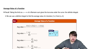
Average Value of a Function

The average value of a continuous function ƒ over an interval [a, b] is calculated using the formula (1/(b-a)) * ∫[a to b] ƒ(x) dx. This concept is essential for determining how the function behaves on the specified interval, providing a single representative value that summarizes the function's overall trend.

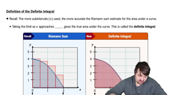
Definite Integral

A definite integral represents the accumulation of quantities, such as area under a curve, over a specific interval. In this context, it is used to compute the integral of the function ƒ(x) = a𝓍(1 - 𝓍) from 0 to 1, which is necessary for finding the average value of the function.

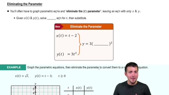
Parameter in Functions

A parameter is a variable that influences the behavior of a function but is not the primary variable of interest. In this case, 'a' is a parameter that affects the shape and scale of the function ƒ(x) = a𝓍(1 - 𝓍), and understanding its role is crucial for expressing the average value as a function of 'a'.

Average value with a parameter Consider the function ƒ(𝓍) = a𝓍 (1―𝓍) on the interval [0, 1], where a is a positive real number.(a) Find the average value of ƒ as a function of a .