Chapter 8: Hypothesis Testing in Statistics – Concepts, Methods, and Applications

Study Guide - Smart Notes

Tailored notes based on your materials, expanded with key definitions, examples, and context.

Section 8: Basics of Hypothesis Testing

Introduction to Hypothesis Testing

Hypothesis testing is a fundamental method in inferential statistics, allowing us to use sample data to make inferences or draw conclusions about a population. This process is essential for evaluating claims or hypotheses about population parameters, such as means or proportions.

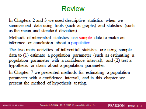
Descriptive statistics summarize data using tools like graphs and measures (mean, standard deviation).
Inferential statistics use sample data to infer or conclude about a population.
Main activities: (1) Estimating population parameters (e.g., confidence intervals), (2) Testing hypotheses about population parameters.

Review of inferential statistics and hypothesis testing

Examples of Hypotheses That Can Be Tested

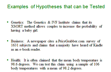
Hypothesis testing is widely used in various fields to evaluate claims based on sample data. Examples include:

Genetics: Testing if a method increases the probability of having a baby girl.
Business: Testing if a majority of people have heard of a product.
Health: Testing if the mean body temperature differs from a commonly believed value.

Examples of hypotheses that can be tested

Conducting a Hypothesis Test

Steps in Hypothesis Testing

To test a claim about a population parameter, follow these structured steps:

Identify the claim and express it in symbolic form.
Write the opposite of the claim in symbolic form.
Formulate hypotheses:
- Null hypothesis (H0): Always contains equality (=).
- Alternative hypothesis (H1): Contains the inequality (<, >, or ≠).
Determine the test type: Left-tailed, right-tailed, or two-tailed, based on the alternative hypothesis.
Identify the parameter: Proportion (p) or mean (μ), and whether population standard deviation (σ) is known.
Choose the significance level (α): Common values are 0.05, 0.01, or 0.10.
Calculate the test statistic: Use z-score or t-score as appropriate.
Find the P-value or critical value and compare with α.
Make a decision: Reject or fail to reject H0.
State the conclusion in context, addressing the original claim.

Formulating Hypotheses

Null Hypothesis (H0): The statement being tested, usually a statement of 'no effect' or 'no difference.' It always includes equality (e.g., μ = μ0).
Alternative Hypothesis (H1): The statement we are trying to find evidence for. It uses <, >, or ≠.

Types of Tests

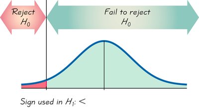
Left-tailed test: H1: parameter < value
Right-tailed test: H1: parameter > value
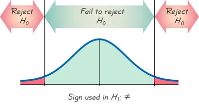
Two-tailed test: H1: parameter ≠ value

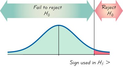
Visualizing Rejection Regions

The rejection region is the area of the sampling distribution where, if the test statistic falls within it, the null hypothesis is rejected.

Two-tailed test: Reject H0 if the test statistic is in either tail.
Left-tailed test: Reject H0 if the test statistic is in the left tail.
Right-tailed test: Reject H0 if the test statistic is in the right tail.

Two-tailed rejection region Left-tailed rejection region Right-tailed rejection region

Methods for Hypothesis Testing

P-value method: Calculate the probability of observing a test statistic as extreme as, or more extreme than, the observed value under H0. If P-value < α, reject H0.
Critical value method: Compare the test statistic to a critical value determined by α. If the test statistic falls in the rejection region, reject H0.

Test Statistics and Calculator Functions

Proportion (p): Use 1-PropZTest
Mean (μ) with unknown σ: Use T-Test
Mean (μ) with known σ: Use Z-Test

Critical Values and Tail Types

Critical values depend on the type of test:

Two-tailed: Use InvNorm(area, 0, 1) or InvT(area, df)
Left-tailed: Use InvNorm(area, 0, 1) or InvT(area, df)
Right-tailed: Use InvNorm(area, 0, 1) or InvT(area, df)

Degrees of freedom (df) are typically n – 1 for a single sample.

Normal distribution curve for critical values

Conclusion Statements

The conclusion of a hypothesis test should be stated in the context of the original claim. The following table summarizes the appropriate wording:

Condition	Conclusion
Original claim does not include equality, and you reject H0	There is sufficient evidence to support the claim that ... (original claim).
Original claim does not include equality, and you fail to reject H0	There is not sufficient evidence to support the claim that ... (original claim).
Original claim does include equality, and you reject H0	There is sufficient evidence to warrant rejection of the claim that ... (original claim).
Original claim does include equality, and you fail to reject H0	There is not sufficient evidence to warrant rejection of the claim that ... (original claim).

Practice Problems: Applying Hypothesis Testing

Example 1: Proportion Test (Majority Preference)

Scenario: In a poll, 806 adults were asked to identify their favorite seat when flying, and 492 chose a window seat. Test the claim that the majority prefer window seats at α = 0.01.

Step 1: Claim in symbols: p > 0.5
Step 2: Opposite: p ≤ 0.5
Step 3: H0: p = 0.5; H1: p > 0.5
Step 4: Right-tailed test
Step 5: Proportion problem (use 1-PropZTest)
Step 6: Calculate P-value and compare to α
Step 7: Decide to reject or fail to reject H0
Step 8: State conclusion in context

Practice problem: majority preference for window seats

Example 2: Proportion Test (Postponing Death)

Scenario: Test the claim that the proportion of deaths in the week before Thanksgiving is less than 0.5 (α = 0.05).

Step 1: Claim in symbols: p < 0.5
Step 2: Opposite: p ≥ 0.5
Step 3: H0: p = 0.5; H1: p < 0.5
Step 4: Left-tailed test
Step 5: Proportion problem (use 1-PropZTest)
Step 6: Calculate P-value and compare to α
Step 7: Decide to reject or fail to reject H0
Step 8: State conclusion in context

Practice problem: proportion of deaths before Thanksgiving

Example 3: Proportion Test (M&Ms Color)

Scenario: In a sample of 100 M&Ms, 8% were brown. Test the claim that the percentage of brown M&Ms is 13% (α = 0.05).

Step 1: Claim in symbols: p = 0.13
Step 2: Opposite: p ≠ 0.13
Step 3: H0: p = 0.13; H1: p ≠ 0.13
Step 4: Two-tailed test
Step 5: Proportion problem (use 1-PropZTest)
Step 6: Calculate P-value and compare to α
Step 7: Decide to reject or fail to reject H0
Step 8: State conclusion in context

Practice problem: percentage of brown M&Ms

Example 4: Mean Test (Body Temperature)

Scenario: A sample of 106 body temperatures has a mean of 98.2°F and a standard deviation of 0.62°F. Test the claim that the mean body temperature is 98.6°F (α = 0.05).

Step 1: Claim in symbols: μ = 98.6
Step 2: Opposite: μ ≠ 98.6
Step 3: H0: μ = 98.6; H1: μ ≠ 98.6
Step 4: Two-tailed test
Step 5: Mean without σ (use T-Test)
Step 6: Calculate P-value and compare to α
Step 7: Decide to reject or fail to reject H0
Step 8: State conclusion in context

Practice problem: mean body temperature

Example 5: Mean Test (Flight Delay Times)

Scenario: The mean departure delay time for 48 flights is 10.5 min (SD = 30.8 min). Test the claim that the mean delay is less than 12.0 min (α = 0.01).

Step 1: Claim in symbols: μ < 12.0
Step 2: Opposite: μ ≥ 12.0
Step 3: H0: μ = 12.0; H1: μ < 12.0
Step 4: Left-tailed test
Step 5: Mean without σ (use T-Test)
Step 6: Calculate P-value and compare to α
Step 7: Decide to reject or fail to reject H0
Step 8: State conclusion in context

Practice problem: mean flight delay times

Example 6: Mean Test (Plastic Waste)

Scenario: The mean weight of discarded plastic from 62 households is 1.911 lb (SD = 1.065 lb). Test the claim that the mean is greater than 1.800 lb (α = 0.05).

Step 1: Claim in symbols: μ > 1.800
Step 2: Opposite: μ ≤ 1.800
Step 3: H0: μ = 1.800; H1: μ > 1.800
Step 4: Right-tailed test
Step 5: Mean without σ (use T-Test)
Step 6: Calculate P-value and compare to α
Step 7: Decide to reject or fail to reject H0
Step 8: State conclusion in context

Practice problem: mean weight of discarded plastic

Example 7: Mean Test (Oscar Winners' Ages)

Scenario: The mean age of 82 Oscar-winning actresses is 35.9 years (σ = 11.1 years). Test the claim that the mean age is 33 years (α = 0.01).

Step 1: Claim in symbols: μ = 33
Step 2: Opposite: μ ≠ 33
Step 3: H0: μ = 33; H1: μ ≠ 33
Step 4: Two-tailed test
Step 5: Mean with σ (use Z-Test)
Step 6: Calculate P-value and compare to α
Step 7: Decide to reject or fail to reject H0
Step 8: State conclusion in context

Practice problem: mean age of Oscar-winning actresses

Example 8: Mean Test (Supermodel Heights)

Scenario: Heights (in inches) of 10 supermodels are given. Test the claim that their mean height is greater than 63.8 in (α = 0.01).

Step 1: Claim in symbols: μ > 63.8
Step 2: Opposite: μ ≤ 63.8
Step 3: H0: μ = 63.8; H1: μ > 63.8
Step 4: Right-tailed test
Step 5: Mean without σ (use T-Test)
Step 6: Calculate P-value and compare to α
Step 7: Decide to reject or fail to reject H0
Step 8: State conclusion in context

Practice problem: mean height of supermodels

Key Formulas

Test statistic for mean (z):
Test statistic for mean (t):
Test statistic for proportion (z):

Note: Use the z-test when the population standard deviation (σ) is known, and the t-test when it is unknown and the sample size is small (n < 30).

Summary Table: Calculator Functions for Hypothesis Testing

Parameter	Calculator Function
Proportion (p)	1-PropZTest
Mean (μ) without σ	T-Test
Mean (μ) with σ	Z-Test