Organizing and Summarizing Data: Introductory Statistics Study Guide

Chapter 2: Organizing and Summarizing Data

2.1 Organizing Qualitative Data

Qualitative data refers to non-numeric information that can be categorized based on attributes or qualities. Proper organization of qualitative data is essential for meaningful analysis and interpretation.

• Frequency Distribution: Lists each category and the number of occurrences for each category.

• Relative Frequency: The proportion or percentage of observations within a category, calculated as: $\text{Relative Frequency} = \frac{\text{Frequency}}{\text{Sum of all frequencies}}$

• Relative Frequency Distribution: Lists each category with its relative frequency.

• Bar Graphs: Visual representation of frequencies or relative frequencies for each category. Bars are of equal width, and their height represents the frequency.

• Pareto Chart: A bar graph with bars arranged in decreasing order of frequency or relative frequency.

• Side-by-Side Bar Graphs: Used to compare data across groups, especially when sample sizes differ. Relative frequencies are preferred for comparison.

• Pie Charts: Circle divided into sectors, each representing a category. The area of each sector is proportional to the frequency.

Example: Survey data on "Best Day of the Week" can be organized into frequency and relative frequency tables, bar graphs, Pareto charts, and pie charts.

2.2 Organizing Quantitative Data: The Popular Displays

Quantitative data consists of numerical values and can be either discrete (countable) or continuous (measurable). The method of organization depends on the type of quantitative data.

• Discrete Data: If few values, use the actual values as classes. If many, group into intervals.

• Continuous Data: Always grouped into intervals called classes.

• Class Limits: Lower class limit is the smallest value in a class; upper class limit is the largest. Class width is the difference between consecutive lower class limits.

• Frequency and Relative Frequency Distributions: Organize data into tables showing counts and proportions for each class.

• Histograms: Rectangles represent classes; height is frequency or relative frequency. Rectangles touch, indicating continuous data.

• Dot Plots: Each observation is plotted as a dot above its value on a horizontal axis.

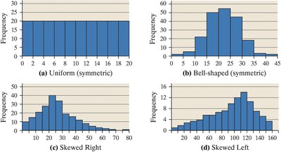
• Distribution Shapes: Describes the pattern of data frequencies:

  • Uniform: Frequencies are evenly spread.

  • Bell-shaped: Highest frequency in the middle, tails off at both ends.

  • Skewed Right: Right tail is longer.

  • Skewed Left: Left tail is longer.

Caution: Qualitative data is not described as skewed or uniform.

Example: Unemployment rates by state can be organized into frequency tables and histograms.

2.3 Additional Displays of Quantitative Data

Beyond histograms and dot plots, several other graphical methods are used to summarize quantitative data.

• Stem-and-Leaf Plots: Digits to the left of the rightmost digit form the stem; rightmost digit forms the leaf. Stems are listed vertically, leaves horizontally.

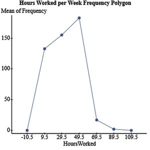
• Frequency Polygons: Points plotted above class midpoints, connected by line segments. Two additional segments connect ends to the horizontal axis. Class Midpoint Formula: $\text{Class Midpoint} = \frac{\text{Lower class limit} + \text{Upper class limit}}{2}$

• Cumulative Frequency Tables: Show the total number of observations less than or equal to each class.

• Cumulative Relative Frequency Tables: Show the proportion of observations less than or equal to each class.

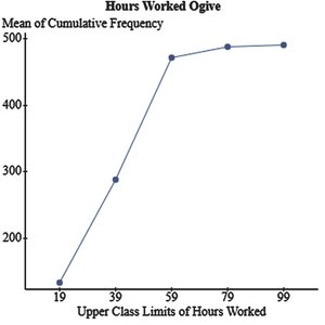
• Ogives: Graphs of cumulative frequency or cumulative relative frequency, plotted at upper class limits.

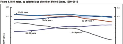
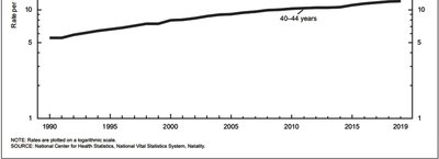
• Time-Series Graphs: Plot values over time, useful for identifying trends.

Example: Frequency polygon and ogive for "Hours Worked" data.

Example: Time-series plots for birth rates by age group and for ages 40-44. These plots help identify which age group has the highest birth rate and trends over time.

2.4 Graphical Misrepresentations of Data

Graphs are powerful tools for communication, but they can be misleading if not constructed carefully.

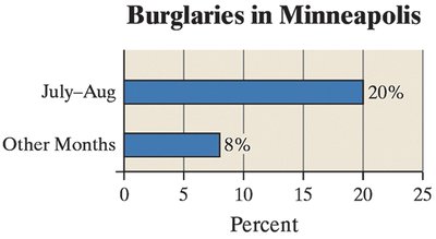
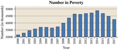
• Misleading Scales: Inconsistent scales or misplaced origins can distort the message.

• Comparative Graphs: Scales should be the same for fair comparison.

• Baseline Assumptions: Readers often assume the baseline is zero; starting at a higher or lower value can mislead.

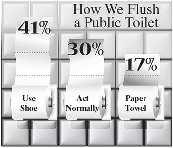
Example: Bar graphs and pictorial graphs can be misleading if the scale or visual representation exaggerates differences.

Summary Table: Types of Graphical Displays

Type of Display	Data Type	Main Purpose
Bar Graph	Qualitative	Compare frequencies/relative frequencies
Pareto Chart	Qualitative	Highlight most frequent categories
Pie Chart	Qualitative	Show proportion of each category
Histogram	Quantitative	Show distribution of data
Dot Plot	Quantitative	Show individual data points
Stem-and-Leaf Plot	Quantitative	Show data distribution and retain original values
Frequency Polygon	Quantitative	Show shape of distribution
Ogive	Quantitative	Show cumulative frequencies
Time-Series Plot	Quantitative (over time)	Show trends over time

Additional info: This guide expands on brief textbook points to provide definitions, examples, formulas, and visual context for each type of data display. It is suitable for exam preparation and self-study in an Introductory Statistics course.