Tabular and Visual Summarization of Variables: Study Guide for Introductory Statistics

Tabular and Visual Summarization of Variables

Introduction to Data Summarization

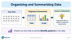
Organizing and summarizing data is a fundamental step in statistics, allowing raw data to be transformed into meaningful information. Summaries can be tabular (tables) or visual (graphs and charts), making patterns and key features easier to identify and interpret.

• Raw Data: Individual observations before any organization.

• Tabular Summary: Data organized into tables for clarity.

• Visual Summary: Data displayed using graphs or charts.

• Purpose: To make data easier to understand and to identify important patterns quickly.

Describing Categorical Data with Tables and Graphs

Categorical Data Organization

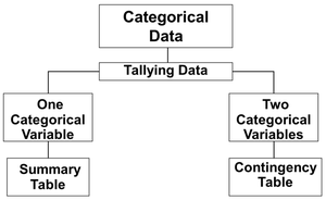
Categorical variables represent qualitative data, such as gender, program, or preferred study method. These are organized using summary tables and contingency tables.

• Summary Table: Shows frequency and percentage for each category of a single categorical variable.

• Contingency Table: Summarizes two categorical variables, displaying frequencies for each combination of categories.

Summary Table Example

For a variable like preferred study method, a summary table lists each category (e.g., Alone, With Friends, Online), the frequency (number of students), and the percentage (frequency divided by total, times 100).

• Formula for Percentage: $\text{Percentage} = \frac{\text{Frequency}}{\text{Total}} \times 100$

Contingency Table Example

A contingency table compares two categorical variables, such as program and gender. It shows the frequency of each combination and can be used to calculate various percentages:

• Overall Percentage: $\text{Overall Percentage} = \frac{\text{Cell Frequency}}{\text{Grand Total}} \times 100$

• Row Percentage: $\text{Row Percentage} = \frac{\text{Cell Frequency}}{\text{Row Total}} \times 100$

• Column Percentage: $\text{Column Percentage} = \frac{\text{Cell Frequency}}{\text{Column Total}} \times 100$

Visualizing Categorical Data

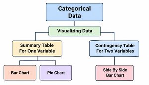
Categorical data can be visualized using bar charts, pie charts, and side-by-side bar charts.

• Bar Chart: Each bar represents a category; height shows frequency or percentage. Bars are separated by gaps.

• Pie Chart: Each slice represents a category; size shows percentage. All slices sum to 100%.

• Side-by-Side Bar Chart: Compares two categories within each group, such as male vs. female students across programs.

Describing Numerical Data with Tables and Graphs

Numerical Data Organization

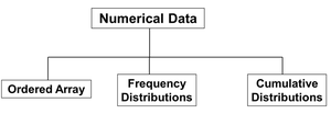
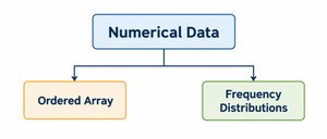
Numerical variables represent quantitative data, such as age or quiz scores. These are organized using ordered arrays and frequency distributions.

• Ordered Array: Data sorted from smallest to largest, showing range and helping identify outliers.

• Frequency Distribution: Data grouped into classes (intervals), showing how many observations fall into each class.

Frequency Distribution Example

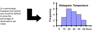
Given quiz scores for 20 students, data are sorted, grouped into classes, and frequencies are counted. Class intervals, midpoints, and boundaries are determined.

Class	Frequency	Relative Frequency	Percentage
10 but less than 20	3	0.15	15%
20 but less than 30	6	0.30	30%
30 but less than 40	5	0.25	25%
40 but less than 50	4	0.20	20%
50 but less than 60	2	0.10	10%
Total	20	1.00	100%

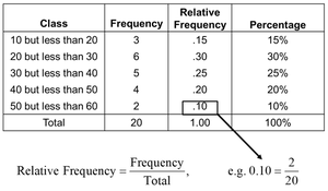
• Relative Frequency Formula: $\text{Relative Frequency} = \frac{\text{Frequency}}{\text{Total}}$

Visualizing Numerical Data

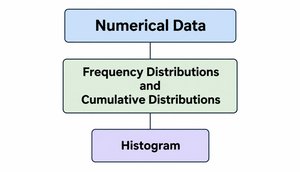
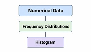
Numerical data are visualized using histograms, which display the distribution of data across intervals.

• Histogram: Bars represent classes; height shows frequency, relative frequency, or percentage. Bars touch because intervals are continuous.

Describing Data for Multiple Variables

Visualizing Two Numerical Variables

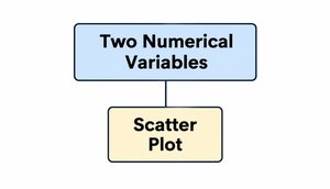
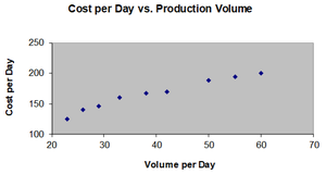
When analyzing two numerical variables, scatter plots are used to visualize their relationship. Each point represents a pair of values.

• Scatter Plot: X-axis shows one variable, Y-axis shows the other. Used to examine relationships between variables.

Correlation Coefficient

The coefficient of correlation quantifies the strength and direction of the linear relationship between two numerical variables.

• Population Correlation Coefficient: Denoted as $\rho$ (rho).

• Sample Correlation Coefficient: Denoted as $r$.

• Properties:

  • Unit free

  • Range: –1 to 1

  • Closer to –1: Strong negative linear relationship

  • Closer to 1: Strong positive linear relationship

  • Closer to 0: Weak linear relationship

Chapter Summary

This chapter covered methods for organizing and visualizing both categorical and numerical variables. Key tools include summary tables, contingency tables, bar charts, pie charts, histograms, and scatter plots. Understanding these methods is essential for effective data analysis in statistics.