Ch. 10 - Chi-Square Tests and the F-Distribution
Larson - Elementary Statistics: Picturing the World 8th Edition
Larson8th EditionElementary Statistics: Picturing the WorldISBN: 9780137493470Not the one you use?Change textbook
Chapter 10, Problem 10.Q.4d

In each exercise,
d. decide whether to reject or fail to reject the null hypothesis, and
[APPLET] In Exercises 3 and 4, use the data, which list the annual wages (in thousands of dollars) for randomly selected individuals from three metropolitan areas. Assume the wages are normally distributed and that the samples are independent. (Adapted from U.S. Bureau of Economic Analysis)
Ithaca, NY: 53.0, 60.3, 34.6, 37.1, 46.6, 46.8, 41.4, 50.6, 50.8, 49.4, 35.0, 36.7, 57.1
Little Rock, AR: 50.7, 43.7, 53.4, 40.0, 45.2, 52.7, 35.2, 60.4, 40.0, 45.9, 45.7, 47.3, 46.5, 44.5, 31.5
Madison, WI: 62.4, 53.9, 67.6, 52.9, 67.7, 50.7, 62.1, 58.9, 61.1, 65.0, 60.4, 59.6, 51.3, 44.8, 66.2
Are the mean annual wages the same for all three cities? Use α=0.10. Assume that the population variances are equal.

Verified step by step guidance
1
Step 1: Define the hypotheses for the ANOVA test. The null hypothesis \(H_0\) states that the mean annual wages are the same for all three cities, i.e., \(\mu_{Ithaca} = \mu_{Little\ Rock} = \mu_{Madison}\). The alternative hypothesis \(H_a\) states that at least one city has a different mean wage.
Step 2: Calculate the sample means and sample variances for each city using the given wage data. This involves summing the wages for each city and dividing by the number of observations to get the means, and then computing the variance for each sample.
Step 3: Compute the overall mean wage by combining all the data from the three cities. This is done by summing all wages from all cities and dividing by the total number of observations.
Step 4: Calculate the Between-Group Sum of Squares (SSB) and the Within-Group Sum of Squares (SSW). Use the formulas: \[SSB = \sum_{i=1}^k n_i (\bar{x}_i - \bar{x})^2\] \[SSW = \sum_{i=1}^k \sum_{j=1}^{n_i} (x_{ij} - \bar{x}_i)^2\] where \(k\) is the number of groups (3 cities), \(n_i\) is the sample size for group \(i\), \(\bar{x}_i\) is the sample mean for group \(i\), and \(\bar{x}\) is the overall mean.
Step 5: Calculate the Mean Squares for Between-Groups (MSB) and Within-Groups (MSW) by dividing the sums of squares by their respective degrees of freedom: \[MSB = \frac{SSB}{k-1}\] \[MSW = \frac{SSW}{N-k}\] where \(N\) is the total number of observations. Then compute the F-statistic: \[F = \frac{MSB}{MSW}\] Finally, compare the calculated F-statistic to the critical value from the F-distribution table at \(\alpha = 0.10\) with degrees of freedom \(k-1\) and \(N-k\). If \(F\) is greater than the critical value, reject the null hypothesis; otherwise, fail to reject it.

Verified video answer for a similar problem:

This video solution was recommended by our tutors as helpful for the problem above.
Video duration:
5m
Was this helpful?

Key Concepts

Here are the essential concepts you must grasp in order to answer the question correctly.

Analysis of Variance (ANOVA)

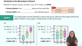
ANOVA is a statistical method used to compare the means of three or more groups to determine if at least one group mean differs significantly. It tests the null hypothesis that all group means are equal by analyzing variance within and between groups. This method is appropriate here since we compare wages across three cities.
Recommended video:
06:46
Introduction to ANOVA

Null and Alternative Hypotheses

The null hypothesis (H0) states that the mean wages are equal across all three cities, while the alternative hypothesis (Ha) claims that at least one city’s mean wage differs. Deciding to reject or fail to reject H0 depends on the ANOVA test results and the chosen significance level (α = 0.10).
Recommended video:
Guided course
06:21
Step 1: Write Hypotheses

Assumption of Equal Population Variances

ANOVA assumes that the populations have equal variances (homogeneity of variance), which affects the validity of the test. This assumption allows pooling of variances to estimate the common variance, making the F-test reliable. The problem explicitly states this assumption, justifying the use of standard ANOVA.
Recommended video:
04:48
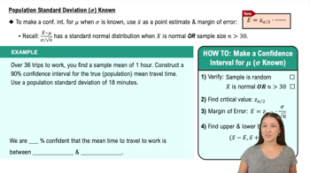
Population Standard Deviation Known
Related Practice
Textbook Question

"In Exercises 13–16, find the critical F-value for a two-tailed test using the level of significance α and degrees of freedom d.f.N and d.f.D.


α=0.05,d.f.N=9,d.f.D=8"

75
views
Textbook Question

In each exercise,

c. find the test statistic,


In Exercises 1 and 2, use the table, which lists the distribution of educational achievement for people in the United States ages 25 and older. It also lists the results of a random survey for two additional age groups. (Adapted from U.S. Census Bureau)


Use the data for 30- to 34-year-olds and 65- to 69-year-olds to test whether age and educational attainment are related. Use α=0.01.

42
views
Textbook Question

In each exercise,

a. identify the claim and state H₀ and Hₐ,


In Exercises 1 and 2, use the table, which lists the distribution of educational achievement for people in the United States ages 25 and older. It also lists the results of a random survey for two additional age groups. (Adapted from U.S. Census Bureau)


Use the data for 30- to 34-year-olds and 65- to 69-year-olds to test whether age and educational attainment are related. Use α=0.01.

43
views
Textbook Question

"In Exercises 9–12, find the critical F-value for a right-tailed test using the level of significance α and degrees of freedom d.f.N and d.f.D.


α=0.05,d.f.N=6,d.f.D=50"

49
views
Textbook Question

In each exercise,

b. find the critical value and identify the rejection region,


In Exercises 1 and 2, use the table, which lists the distribution of educational achievement for people in the United States ages 25 and older. It also lists the results of a random survey for two additional age groups. (Adapted from U.S. Census Bureau)


Use the data for 30- to 34-year-olds and 65- to 69-year-olds to test whether age and educational attainment are related. Use α=0.01.

38
views
Textbook Question

In each exercise,

e. interpret the decision in the context of the original claim.

[APPLET] In Exercises 3 and 4, use the data, which list the annual wages (in thousands of dollars) for randomly selected individuals from three metropolitan areas. Assume the wages are normally distributed and that the samples are independent. (Adapted from U.S. Bureau of Economic Analysis)

Ithaca, NY: 53.0, 60.3, 34.6, 37.1, 46.6, 46.8, 41.4, 50.6, 50.8, 49.4, 35.0, 36.7, 57.1

Little Rock, AR: 50.7, 43.7, 53.4, 40.0, 45.2, 52.7, 35.2, 60.4, 40.0, 45.9, 45.7, 47.3, 46.5, 44.5, 31.5

Madison, WI: 62.4, 53.9, 67.6, 52.9, 67.7, 50.7, 62.1, 58.9, 61.1, 65.0, 60.4, 59.6, 51.3, 44.8, 66.2

Are the mean annual wages the same for all three cities? Use α=0.10. Assume that the population variances are equal.

24
views