Quantitative Genetics: Mapping Additive Alleles with QTLs and GWAS

Quantitative Genetics and Additive Alleles

Introduction to Quantitative Traits

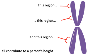
Quantitative traits are phenotypes that show continuous variation (such as height, weight, or yield) and are typically influenced by multiple genes, each contributing additively to the trait. Unlike Mendelian traits, which are controlled by a single gene, quantitative traits result from the combined effect of many genes and environmental factors.

• Quantitative Trait: A trait that varies continuously and is usually influenced by several genes (polygenic) and environmental factors.

• Additive Genes: Genes whose effects on a trait add up to influence the phenotype.

• Example: Human height is determined by the additive effects of many genes, each contributing a small amount to the overall phenotype.

Mapping Additive Alleles: Quantitative Trait Loci (QTLs)

What is a Quantitative Trait Locus (QTL)?

A Quantitative Trait Locus (QTL) is a specific region on a chromosome that is associated with variation in a quantitative trait. QTLs are identified by their statistical association with phenotypic variation in a population.

• QTL: A locus (chromosomal region) that contributes to the variation of a quantitative trait.

• QTLs can be mapped to specific regions of chromosomes using genetic markers.

• Each QTL may explain a portion of the total phenotypic variance for a trait.

Case Study: QTL Mapping in Tomatoes

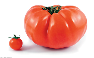
QTL mapping can be used to identify regions of the genome that control important agricultural traits, such as fruit size and shape in tomatoes. By crossing parents with extreme phenotypes and analyzing their offspring, researchers can locate QTLs responsible for these traits.

• More than 28 QTLs have been identified for fruit shape and weight in tomatoes.

• A specific gene (e.g., ORFX) may account for a significant portion (e.g., 30%) of the variation in fruit weight.

QTL Mapping Crosses

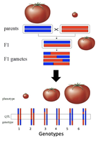
To map QTLs, researchers often start with purebred parental lines that differ in the trait of interest. These are crossed to produce F1 hybrids, which are then interbred or backcrossed to generate recombinant offspring. The genotypes and phenotypes of these offspring are analyzed to identify chromosomal regions associated with the trait.

• Parental lines: One with large fruit, one with small fruit.

• F1 generation: Heterozygous for the trait.

• Recombinant offspring: Show a range of phenotypes due to different combinations of parental alleles.

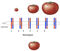
Identifying QTLs Using Genetic Markers

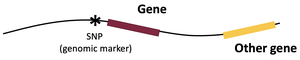
QTLs are identified by associating genetic markers with phenotypic variation. Markers such as Single Nucleotide Polymorphisms (SNPs) are used to distinguish between different chromosomal regions inherited from each parent.

• Genetic Marker: A DNA sequence with a known location that can be used to track inheritance.

• SNP (Single Nucleotide Polymorphism): A single base pair change in the DNA sequence that serves as a unique marker.

• Markers are not usually the cause of the trait but are physically linked to the causal gene.

Using SNPs to Identify QTLs

SNPs are widely used as genetic markers in QTL mapping. They are single base pair differences in the DNA sequence that can be used to distinguish between different alleles. SNPs are typically not the causal variant but are closely linked to the gene affecting the trait.

• SNPs allow researchers to track the inheritance of chromosomal regions in offspring.

• By correlating SNP genotypes with phenotypes, QTLs can be mapped to specific regions of the genome.

QTL Mapping with Introgression Lines (ILs)

Introgression Lines and Fine Mapping

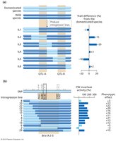
Introgression lines (ILs) are developed by repeated backcrossing and selfing, resulting in lines that are genetically identical except for a small chromosomal segment from a donor parent. ILs are used to fine-map QTLs and identify the specific genes responsible for trait variation.

• ILs allow for precise localization of QTLs by comparing phenotypes across lines with different introgressed segments.

• Trait differences between ILs and the recurrent parent indicate the presence of a QTL in the introgressed region.

Zooming in on QTLs

Once a QTL region is identified, additional ILs can be created to further narrow down the region and identify candidate genes. Sequencing these lines can reveal mutations responsible for the trait.

• Fine mapping increases the resolution of QTL mapping.

• Candidate genes can be tested for their effect on the trait.

Genome-Wide Association Studies (GWAS)

Principles of GWAS

Genome-Wide Association Studies (GWAS) analyze natural populations to identify associations between genetic markers (usually SNPs) and phenotypic traits. Unlike QTL mapping, which uses controlled crosses, GWAS examines genetic variation in unrelated individuals.

• GWAS compares the genomes of individuals with and without a trait (cases vs. controls).

• Statistical analysis identifies SNPs that are significantly associated with the trait.

• The associated SNP is called a "GWAS SNP"; the actual DNA change causing the trait is the "causal variant."

Key distinction: The GWAS SNP is a marker linked to the trait, while the causal variant is the actual genetic change responsible for the phenotype.

GWAS Example: Crohn’s Disease

GWAS has been used to identify genetic regions associated with Crohn’s disease, an intestinal disorder influenced by inherited variation. By comparing SNP frequencies in affected individuals (cases) and unaffected individuals (controls), researchers can pinpoint genomic regions linked to disease susceptibility.

• Significant associations are visualized using a Manhattan plot, where peaks indicate genomic regions with strong statistical association.

• For Crohn’s disease, notable peaks are found on chromosomes 6 and X, among others.

Genetic and Environmental Contributions to Quantitative Traits

Partitioning Phenotypic Variance

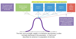
The variation observed in quantitative traits is due to both genetic and environmental factors. The total phenotypic variance (VP) can be partitioned into genetic variance (VG), environmental variance (VE), and sometimes gene-environment interaction variance (VGE).

• VP = VG + VE + VGE

• Genetic variance can be further divided into additive, dominance, and epistatic components.

• Quantitative traits often show a normal (bell-shaped) distribution in populations due to the combined effects of many genes and environmental influences.

Summary Table: QTL Mapping vs. GWAS

Feature	QTL Mapping	GWAS
Population	Controlled crosses (e.g., F2, backcross, ILs)	Natural populations
Markers	SNPs, other genetic markers	SNPs
Resolution	Moderate (depends on recombination events)	High (many recombination events in population history)
Detects	Chromosome regions linked to trait	Statistical association between SNPs and trait
Limitation	Limited to variation between parents	Population structure can confound results

Additional info: The study of quantitative genetics is essential for understanding complex traits in agriculture, medicine, and evolutionary biology. Both QTL mapping and GWAS are powerful tools for dissecting the genetic architecture of these traits.