Ch. 4 - Discrete Probability Distributions
Larson - Elementary Statistics: Picturing the World 8th Edition
Larson8th EditionElementary Statistics: Picturing the WorldISBN: 9780137493470Not the one you use?Change textbook
Chapter 4, Problem 4.2.27

Constructing and Graphing Binomial Distributions In Exercises 27–30, (a) construct a binomial distribution, (b) graph the binomial distribution using a histogram and describe its shape, and (c) identify any values of the random variable x that you would consider unusual. Explain your reasoning.


College Acceptance Pennsylvania State University accepts 49% of applicants. You randomly select seven Pennsylvania State University applicants. The random variable represents the number who are accepted. (Source: US News & World Report)

Verified step by step guidance
1
Step 1: Understand the problem and identify the parameters of the binomial distribution. A binomial distribution is defined by two parameters: the number of trials (n) and the probability of success (p). Here, n = 7 (the number of applicants selected) and p = 0.49 (the probability of an applicant being accepted). The random variable x represents the number of applicants accepted.
Step 2: Construct the binomial distribution. Use the binomial probability formula to calculate the probability for each possible value of x (from 0 to 7). The formula is: P(x) = (n choose x) * p^x * (1-p)^(n-x), where (n choose x) = n! / [x! * (n-x)!]. Compute P(x) for x = 0, 1, 2, ..., 7.
Step 3: Create a histogram to graph the binomial distribution. Plot the values of x (0 through 7) on the horizontal axis and their corresponding probabilities P(x) on the vertical axis. Label the axes clearly and ensure the bars represent the probabilities accurately.
Step 4: Describe the shape of the distribution. Analyze the histogram to determine whether the distribution is symmetric, skewed left, or skewed right. For a binomial distribution with p close to 0.5 and a small n, the shape is often approximately symmetric.
Step 5: Identify unusual values of x. In statistics, a value is considered unusual if its probability is less than 0.05. Examine the probabilities P(x) calculated in Step 2 and identify any x values with probabilities below this threshold. Explain why these values are considered unusual based on their low likelihood of occurrence.

Verified video answer for a similar problem:

This video solution was recommended by our tutors as helpful for the problem above.
Video duration:
5m
Was this helpful?

Key Concepts

Here are the essential concepts you must grasp in order to answer the question correctly.

Binomial Distribution

A binomial distribution models the number of successes in a fixed number of independent Bernoulli trials, each with the same probability of success. In this context, the random variable represents the number of applicants accepted from a sample of seven, where each applicant has a 49% chance of being accepted. The distribution is defined by two parameters: the number of trials (n) and the probability of success (p).
Recommended video:
Guided course
03:28
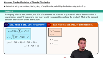
Mean & Standard Deviation of Binomial Distribution

Histogram

A histogram is a graphical representation of the distribution of numerical data, where the data is divided into bins or intervals. In the case of a binomial distribution, the histogram will display the frequency of each possible outcome (number of accepted applicants) on the x-axis, with the height of the bars representing the probability of each outcome. This visual tool helps in understanding the shape and spread of the distribution.
Recommended video:
Guided course
05:54
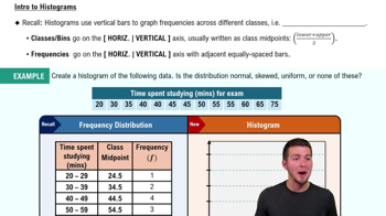
Intro to Histograms

Unusual Values

Unusual values in a distribution are those that lie significantly outside the expected range of outcomes, often defined as values that fall beyond two standard deviations from the mean. In the context of the binomial distribution for this problem, identifying unusual values involves analyzing the probabilities of extreme outcomes (like 0 or 7 accepted applicants) and determining if they are significantly lower or higher than what would be expected based on the distribution.
Recommended video:
Guided course
06:50
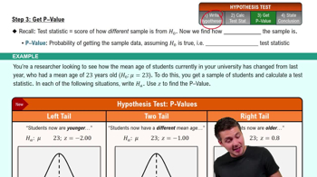
Step 3: Get P-Value
Related Practice
Textbook Question

Finding Binomial Probabilities In Exercises 19–26, find the indicated probabilities. If convenient, use technology or Table 2 in Appendix B.


Penalty Kicks Argentine soccer player Lionel Messi converts 78% of his penalty kicks. Suppose Messi takes six penalty kicks next season. Find the probability that the number he converts is (a) exactly six, (b) at most three, and (c) more than three. (Source: Transfermarkt)

99
views
Textbook Question

Graphical Analysis In Exercises 9–12, determine whether the graph on the number line represents a discrete random variable or a continuous random variable. Explain your reasoning.


The attendance at concerts for a rock group

95
views
Textbook Question

Identifying and Understanding Binomial Experiments In Exercises 15–18, determine whether the experiment is a binomial experiment. If it is, identify a success; specify the values of n, p, and q; and list the possible values of the random variable x. If it is not a binomial experiment, explain why.


Video Games A survey found that 29% of gamers own a virtual reality (VR) device. Ten gamers are randomly selected. The random variable represents the number who own a VR device. (Source: Entertainment Software Association)

111
views
Textbook Question

True or False? In Exercises 5–8, determine whether the statement is true or false. If it is false, rewrite it as a true statement.


For a random variable x, the word random indicates that the value of x is determined by chance.

103
views
Textbook Question

Discrete Variables and Continuous Variables In Exercises 13–18, determine whether the random variable x is discrete or continuous. Explain.


Let x represent the length of time it takes to complete an exam.

62
views
Textbook Question

Finding the Mean, Variance, and Standard Deviation In Exercises 29–34, (a) find the mean, variance, and standard deviation of the probability distribution, and (b) interpret the results.

Machine Parts The number of defects per 1000 machine parts inspected

84
views