Ch. 6 - Normal Probability Distributions
Triola - Elementary Statistics 14th Edition
Triola14th EditionElementary StatisticsISBN: 9780137366446Not the one you use?Change textbook
Chapter 6, Problem 6.5.1

Satisfying Requirements Data Set 1 “Body Data” in Appendix B includes a sample of 147 pulse rates of randomly selected women. Does that sample satisfy the following requirement: (1) The sample appears to be from a normally distributed population; or (2) the sample has a size of n>30?

Verified step by step guidance
1
Step 1: To determine if the sample appears to be from a normally distributed population, create a histogram or a normal probability plot of the pulse rates. A histogram should show a bell-shaped curve, and a normal probability plot should display points that closely follow a straight line.
Step 2: Perform a statistical test for normality, such as the Shapiro-Wilk test or the Kolmogorov-Smirnov test, using the pulse rate data. These tests provide a p-value to assess whether the data significantly deviates from a normal distribution.
Step 3: Evaluate the sample size condition. The problem states that the sample size is 147, which is greater than 30. This satisfies the requirement for n > 30.
Step 4: Combine the results from the normality assessment and the sample size evaluation. If the data is approximately normal or the sample size is sufficiently large (n > 30), the sample can be considered valid for statistical analysis.
Step 5: Document your findings clearly, noting whether the sample satisfies each requirement based on the analysis performed in the previous steps.

Verified video answer for a similar problem:

This video solution was recommended by our tutors as helpful for the problem above.
Video duration:
3m
Was this helpful?

Key Concepts

Here are the essential concepts you must grasp in order to answer the question correctly.

Normal Distribution

Normal distribution is a probability distribution that is symmetric about the mean, showing that data near the mean are more frequent in occurrence than data far from the mean. In statistics, many tests and methods assume that the data follows a normal distribution, which is characterized by its bell-shaped curve. Understanding whether a sample is normally distributed is crucial for applying certain statistical techniques.
Recommended video:
Guided course
09:47
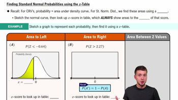
Finding Standard Normal Probabilities using z-Table

Sample Size and Central Limit Theorem

The Central Limit Theorem states that, for a sufficiently large sample size (typically n > 30), the sampling distribution of the sample mean will be approximately normally distributed, regardless of the shape of the population distribution. This theorem justifies the use of normal distribution methods for larger samples, making it essential to consider sample size when analyzing data.
Recommended video:
04:08
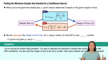
Finding the Minimum Sample Size Needed for a Confidence Interval

Statistical Inference

Statistical inference involves using data from a sample to make conclusions about a larger population. It includes methods such as hypothesis testing and confidence intervals, which rely on the assumptions of normality and sample size. Understanding these concepts is vital for determining the validity of the conclusions drawn from the sample data.
Recommended video:
Guided course
05:53
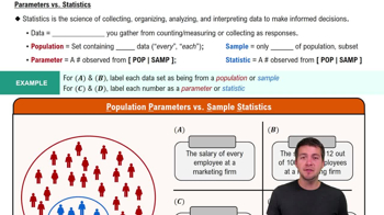
Parameters vs. Statistics
Related Practice
Textbook Question

Basis for the Range Rule of Thumb and the Empirical Rule. In Exercises 45–48, find the indicated area under the curve of the standard normal distribution; then convert it to a percentage and fill in the blank. The results form the basis for the range rule of thumb and the empirical rule introduced in Section 3-2.


About __ % of the area is between z = -1 and z = 1 (or within 1 standard deviation of the mean).

163
views
Textbook Question

Finding Bone Density Scores. In Exercises 37–40 assume that a randomly selected subject is given a bone density test. Bone density test scores are normally distributed with a mean of 0 and a standard deviation of 1. In each case, draw a graph, then find the bone density test score corresponding to the given information. Round results to two decimal places.


Find the bone density scores that are the quartiles Q1, Q2, and Q3.

136
views
Textbook Question

Pulse Rates. In Exercises 13–24, use the data in the table below for pulse rates of adult males and females (based on Data Set 1 “Body Data” in Appendix B). Hint: Draw a graph in each case.


" style="" width="340">


Find the probability that a male has a pulse rate between 70 beats per minute and 90 beats per minute.

390
views
Textbook Question

Standard Normal Distribution. In Exercises 17–36, assume that a randomly selected subject is given a bone density test. Those test scores are normally distributed with a mean of 0 and a standard deviation of 1. In each case, draw a graph, then find the probability of the given bone density test scores. If using technology instead of Table A-2, round answers to four decimal places.


Less than -2.00

207
views
Textbook Question

Continuous Uniform Distribution. In Exercises 5–8, refer to the continuous uniform distribution depicted in Figure 6-2 and described in Example 1. Assume that a passenger is randomly selected, and find the probability that the waiting time is within the given range.


" style="" width="225">


Greater than 3.00 minutes

363
views
Textbook Question

Pulse Rates. In Exercises 13–24, use the data in the table below for pulse rates of adult males and females (based on Data Set 1 “Body Data” in Appendix B). Hint: Draw a graph in each case.


" style="" width="340">


For males, find P90 which is the pulse rate separating the bottom 90% from the top 10%.

271
views