Ch. 9 - Differential Equations
Briggs - Calculus: Early Transcendentals 3rd Edition
Briggs3rd EditionCalculus: Early TranscendentalsISBN: 9780136847243Not the one you use?Change textbook
Chapter 9, Problem 9.2.21

21–24. Logistic equations Consider the following logistic equations. In each case, sketch the direction field, draw the solution curve for each initial condition, and find the equilibrium solutions. A detailed direction field is not needed. Assume t ≥ 0 and tP ≥ 0.
P′(t) = 0.05P(1−P/800); P(0) = 100, P(0) = 400, P(0) = 700

Verified step by step guidance
1
Identify the given logistic differential equation: \(P\'(t) = 0.05P\left(1 - \frac{P}{800}\right)\), where \(P(t)\) represents the population at time \(t\).
Find the equilibrium solutions by setting the derivative equal to zero: \(0 = 0.05P\left(1 - \frac{P}{800}\right)\). Solve for \(P\) to find the constant solutions where the population does not change.
Analyze the stability of each equilibrium by considering the sign of \(P\'(t)\) for values of \(P\) slightly less than and greater than each equilibrium. This helps understand whether solutions move towards or away from these points.
Sketch the direction field by plotting small slope segments at various points \((t, P)\) based on the value of \(P\'(t)\). Since \(t \geq 0\) and \(P \geq 0\), focus on this region. The slope at each point is given by the right-hand side of the differential equation.
Draw solution curves starting from the initial conditions \(P(0) = 100\), \(P(0) = 400\), and \(P(0) = 700\). Use the direction field and the logistic growth behavior to sketch how the population evolves over time, approaching the equilibrium solutions.

Verified video answer for a similar problem:

This video solution was recommended by our tutors as helpful for the problem above.
Video duration:
3m
Was this helpful?

Key Concepts

Here are the essential concepts you must grasp in order to answer the question correctly.

Logistic Differential Equation

A logistic differential equation models population growth with a carrying capacity, balancing growth and limiting factors. It has the form P'(t) = rP(1 - P/K), where r is the growth rate and K is the carrying capacity. This equation produces an S-shaped curve, showing initial exponential growth that slows as the population approaches K.
Recommended video:
07:39
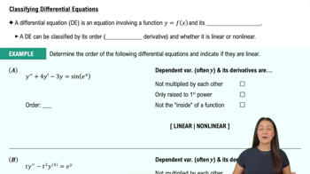
Classifying Differential Equations

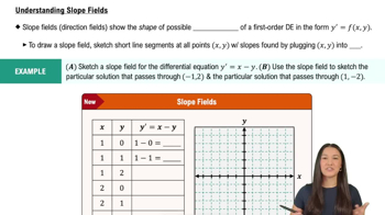
Direction Fields (Slope Fields)

Direction fields graphically represent the slopes of solutions to differential equations at various points. Each small line segment indicates the slope of the solution curve at that point, helping visualize behavior without solving analytically. For logistic equations, direction fields show how solutions evolve over time from different initial conditions.
Recommended video:
05:45
Understanding Slope Fields

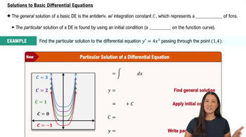
Equilibrium Solutions

Equilibrium solutions occur where the derivative P'(t) equals zero, meaning the population remains constant over time. For logistic equations, these are typically at P = 0 and P = K, representing extinction and carrying capacity. Stability analysis of these points helps understand long-term population behavior.
Recommended video:
04:00
Solutions to Basic Differential Equations