Ch. 10 - Correlation and Regression

Triola - Elementary Statistics 14th Edition

Triola14th EditionElementary StatisticsISBN: 9780137366446Not the one you use?Change textbook

Triola 14th Edition

Ch. 10 - Correlation and Regression

Problem 10.2.4

Chapter 10, Problem 10.2.4

Correlation and Slope What is the relationship between the linear correlation coefficient r and the slope b1 of a regression line?

Verified step by step guidance

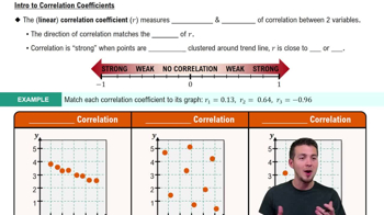
The linear correlation coefficient, denoted as r, measures the strength and direction of the linear relationship between two variables. It ranges from -1 to 1, where values close to -1 or 1 indicate a strong linear relationship, and values near 0 indicate a weak or no linear relationship.

The slope of the regression line, denoted as b₁, represents the rate of change in the dependent variable (y) for a one-unit increase in the independent variable (x). It is calculated as b₁ = r * (sy / sx), where sy and sx are the standard deviations of y and x, respectively.

The relationship between r and b₁ is that the sign of r (positive or negative) determines the direction of the slope b₁. If r is positive, b₁ will also be positive, indicating an upward-sloping line. If r is negative, b₁ will be negative, indicating a downward-sloping line.

The magnitude of r affects the strength of the linear relationship but does not directly determine the value of b₁. The value of b₁ also depends on the variability (standard deviations) of the variables x and y.

In summary, while r and b₁ are related through the formula b₁ = r * (sy / sx), they describe different aspects of the relationship: r quantifies the strength and direction of the correlation, while b₁ quantifies the rate of change in y with respect to x.

Verified video answer for a similar problem:

This video solution was recommended by our tutors as helpful for the problem above.

Video duration:

Was this helpful?

Key Concepts

Here are the essential concepts you must grasp in order to answer the question correctly.

Linear Correlation Coefficient (r)

The linear correlation coefficient, denoted as r, measures the strength and direction of a linear relationship between two variables. Its value ranges from -1 to 1, where -1 indicates a perfect negative correlation, 1 indicates a perfect positive correlation, and 0 indicates no correlation. Understanding r is crucial for interpreting how closely two variables are related.

Slope of a Regression Line (b1)

The slope of a regression line, represented as b1, quantifies the change in the dependent variable for each unit change in the independent variable. A positive slope indicates that as the independent variable increases, the dependent variable also increases, while a negative slope indicates the opposite. The slope is a key component in understanding the nature of the relationship modeled by the regression.

Relationship Between r and b1

The relationship between the linear correlation coefficient r and the slope b1 is significant in regression analysis. Specifically, when both variables are standardized, the slope b1 is equal to the correlation coefficient r. This means that a strong correlation (high absolute value of r) typically corresponds to a steep slope, indicating a strong linear relationship between the variables.

Recommended video:

Guided course

03:50

Probabilities Between Two Values

Related Practice

Textbook Question

Super Bowl and R^2 Let x represent years coded as 1,1,3,... for years starting in 1980, and let y represent the numbers of points scored in each annual Super Bowl beginning in 1980. Using the data from 1980 to the last Super Bowl at the time of this writing, we obtain the following values of R^2 for the different models: linear: 0.008; quadratic: 0.023; logarithmic: 0.0004; exponential: 0.027; power: 0.007. Based on these results, which model is best? Is the best model a good model? What do the results suggest about predicting the number of points scored in a future Super Bowl game?

views

Textbook Question

Finding the Best Model

In Exercises 5–16, construct a scatterplot and identify the mathematical model that best fits the given data. Assume that the model is to be used only for the scope of the given data, and consider only linear, quadratic, logarithmic, exponential, and power models.

CD Yields The table lists the value y (in dollars) of \$1000 deposited in a certificate of deposit at Bank of New York (based on rates currently in effect).

views

Textbook Question

Moore’s Law In 1965, Intel cofounder Gordon Moore initiated what has since become known as Moore’s law: The number of transistors per square inch on integrated circuits will double approximately every 18 months. In the table below, the first row lists different years and the second row lists the number of transistors (in thousands) for different years.

Ignoring the listed data and assuming that Moore’s law is correct and transistors per square inch double every 18 months, which mathematical model best describes this law: linear, quadratic, logarithmic, exponential, power? What specific function describes Moore’s law?

Which mathematical model best fits the listed sample data?

Compare the results from parts (a) and (b). Does Moore’s law appear to be working reasonably well?

views

Textbook Question

Large Data Sets

Exercises 29–32 use the same Appendix B data sets as Exercises 29–32 in Section 10-1. In each case, find the regression equation, letting the first variable be the predictor (x) variable. Find the indicated predicted values following the prediction procedure summarized in Figure 10-5.

Taxis Repeat Exercise 16 using all of the distance/tip data from the 703 taxi rides listed in Data Set 32 “Taxis” from Appendix B.

212

views

Textbook Question

Interpreting the Coefficient of Determination

In Exercises 5–8, use the value of the linear correlation coefficient r to find the coefficient of determination and the percentage of the total variation that can be explained by the linear relationship between the two variables.

Times of Taxi Rides and Tips r = 0.298 (x = time in minutes, y = the amount of tip in dollars)

186

views

Textbook Question

Regression and Predictions

Exercises 13–28 use the same data sets as Exercises 13–28 in Section 10-1.

Find the regression equation, letting the first variable be the predictor (x) variable.

Find the indicated predicted value by following the prediction procedure summarized in Figure 10-5.

Oscars Listed below are ages of recent Oscar winners matched by the years in which the awards were won (from Data Set 21 “Oscar Winner Age” in Appendix B). Find the best predicted age of an Oscar-winning actress given that the Oscar winner for best actor is 59 years of age. How does the result compare to the actual actress age of 60 years?

[IMAGE]

202

views