Ch. 10 - Correlation and Regression

Triola - Elementary Statistics 14th Edition

Triola14th EditionElementary StatisticsISBN: 9780137366446Not the one you use?Change textbook

Triola 14th Edition

Ch. 10 - Correlation and Regression

Problem 10.5.6

Chapter 10, Problem 10.5.6

Finding the Best Model
In Exercises 5–16, construct a scatterplot and identify the mathematical model that best fits the given data. Assume that the model is to be used only for the scope of the given data, and consider only linear, quadratic, logarithmic, exponential, and power models.
Dirt Cheap The Cherry Hill Construction company in Branford, CT sells screened topsoil by the “yard,” which is actually a cubic yard. Let the variable x be the length (yd) of each side of a cube of screened topsoil. The table below lists the values of x along with the corresponding cost (dollars).

Verified step by step guidance

Step 1: Begin by plotting the given data points on a scatterplot. Use the variable x (length of each side of the cube in yards) as the independent variable on the x-axis and the cost (in dollars) as the dependent variable on the y-axis.

Step 2: Observe the pattern of the data points on the scatterplot. Determine whether the relationship between x and cost appears to be linear, quadratic, logarithmic, exponential, or power-based. Look for trends such as curvature, rapid growth, or proportional scaling.

Step 3: Fit each of the potential models (linear, quadratic, logarithmic, exponential, and power) to the data using regression techniques. For example, use the least squares method to calculate the coefficients for each model.

Step 4: Evaluate the goodness-of-fit for each model using statistical measures such as the coefficient of determination (R²). The model with the highest R² value is likely the best fit for the data.

Step 5: Once the best-fitting model is identified, write down its mathematical equation. Ensure that the model is only used within the scope of the given data, as extrapolation beyond the provided range may lead to inaccuracies.

Verified video answer for a similar problem:

This video solution was recommended by our tutors as helpful for the problem above.

Video duration:

Was this helpful?

Key Concepts

Here are the essential concepts you must grasp in order to answer the question correctly.

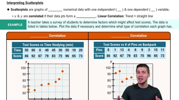
Scatterplot

A scatterplot is a graphical representation of two variables, where each point represents an observation in the dataset. In this context, the x-axis represents the length of the cube of topsoil, while the y-axis represents the corresponding cost. Analyzing the scatterplot helps identify the relationship between the variables and the potential mathematical model that fits the data.

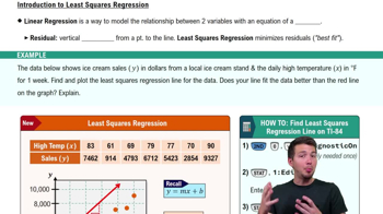
Mathematical Models

Mathematical models are equations that describe the relationship between variables. In this exercise, you are tasked with identifying the best-fitting model from linear, quadratic, logarithmic, exponential, and power models. Each model has distinct characteristics and is suitable for different types of data patterns, making it essential to choose the one that accurately represents the observed relationship.

Cost and Volume Relationship

The relationship between cost and volume in this scenario is influenced by the cubic nature of the topsoil. As the length of each side of the cube increases, the volume—and consequently the cost—grows at a rate that may not be linear. Understanding this relationship is crucial for selecting the appropriate mathematical model that reflects how cost escalates with increasing volume.

Recommended video:

05:06

Finding Probabilities Using the Poisson Distribution Example 2

Related Practice

Textbook Question

Finding the Best Model

In Exercises 5–16, construct a scatterplot and identify the mathematical model that best fits the given data. Assume that the model is to be used only for the scope of the given data, and consider only linear, quadratic, logarithmic, exponential, and power models.

Stock Market Listed below in order by row are the annual high values of the Dow Jones Industrial Average for each year beginning with 2000. Find the best model and then predict the value for the last year listed. Is the predicted value close to the actual value of 26,828.4?

views

Textbook Question

Making Predictions

In Exercises 5–8, let the predictor variable x be the first variable given. Use the given data to find the regression equation and the best predicted value of the response variable. Be sure to follow the prediction procedure summarized in Figure 10-5. Use a 0.05 significance level.

Bear Measurements Head widths (in.) and weights (lb) were measured for 20 randomly selected bears (from Data Set 18 “Bear Measurements” in Appendix B). The 20 pairs of measurements yield xbar = 6.9 in., ybar = 214.3 lb, r = 0.879 P-value = 0.000 and y^ = -212 + 61.9x. Find the best predicted weight of a bear given that the bear has a head width of 6.5 in.

105

views

Textbook Question

Testing for a Linear Correlation

In Exercises 13–28, construct a scatterplot, and find the value of the linear correlation coefficient r. Also find the P-value or the critical values of r from Table A-6. Use a significance level of α = 0.05. Determine whether there is sufficient evidence to support a claim of a linear correlation between the two variables. (Save your work because the same data sets will be used in Section 10-2 exercises.)

Taxis The table below includes data from New York City taxi rides (from Data Set 32 “Taxis” in Appendix B). The distances are in miles, the times are in minutes, the fares are in dollars, and the tips are in dollars. Is there sufficient evidence to support the claim that there is a linear correlation between the time of the ride and the tip amount? Does it appear that riders base their tips on the time of the ride?

157

views

Textbook Question

Testing for a Linear Correlation

Taxis Using the data from Exercise 15, is there sufficient evidence to support the claim that there is a linear correlation between the distance of the ride and the tip amount? Does it appear that riders base their tips on the distance of the ride?

190

views

Textbook Question

Interpreting a Computer Display

In Exercises 5–8, we want to consider the correlation between heights of fathers and mothers and the heights of their sons. Refer to the StatCrunch display and answer the given questions or identify the indicated items. The display is based on Data Set 10 “Family Heights” in Appendix B. (The response y variable represents heights of sons.)

[IMAGE]

Height of Son Should the multiple regression equation be used for predicting the height of a son based on the height of his father and mother? Why or why not?

169

views

Textbook Question

Variation and Prediction Intervals

In Exercises 17–20, find the (a) explained variation, (b) unexplained variation, and (c) indicated prediction interval. In each case, there is sufficient evidence to support a claim of a linear correlation, so it is reasonable to use the regression equation when making predictions.

Weighing Seals with a Camera The table below lists overhead widths (cm) of seals measured from photographs and the weights (kg) of the seals (based on “Mass Estimation of Weddell Seals Using Techniques of Photogrammetry,” by R. Garrott of Montana State University). For the prediction interval, use a 99% confidence level with an overhead width of 9.0 cm.

108

views