Textbook Question
17–32. Solving initial value problems Determine whether the following equations are separable. If so, solve the initial value problem.
y'(t) = y³sin t, y(0) = 1
59
views
 Verified step by step guidance
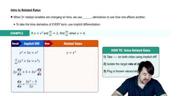
 04:16
04:16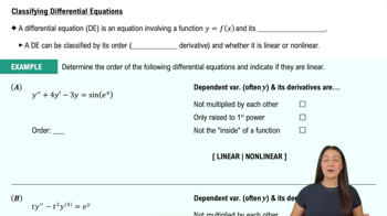 07:39
07:39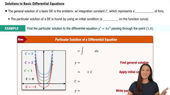 04:00
04:0017–32. Solving initial value problems Determine whether the following equations are separable. If so, solve the initial value problem.
y'(t) = y³sin t, y(0) = 1
7–16. Verifying general solutions Verify that the given function is a solution of the differential equation that follows it. Assume C, C1, C2 and C3 are arbitrary constants.
u(t) = C₁eᵗ + C₂teᵗ; u''(t) - 2u'(t) + u(t) = 0
The general solution of a first-order linear differential equation is y(t) = Ce⁻¹⁰ᵗ − 13. What solution satisfies the initial condition y(0) = 4?
9–14. Growth rate functions Make a sketch of the population function P (as a function of time) that results from the following growth rate functions. Assume the population at time t = 0 begins at some positive value.
9–14. Growth rate functions Make a sketch of the population function P (as a function of time) that results from the following growth rate functions. Assume the population at time t = 0 begins at some positive value.
45–48. General first-order linear equations Consider the general first-order linear equation y'(t)+a(t)y(t)=f(t). This equation can be solved, in principle, by defining the integrating factor p(t)=exp(∫a(t)dt). Here is how the integrating factor works. Multiply both sides of the equation by p (which is always positive) and show that the left side becomes an exact derivative. Therefore, the equation becomes
p(t)(y′(t) + a(t)y(t)) = d/dt(p(t)y(t)) = p(t)f(t).
Now integrate both sides of the equation with respect to t to obtain the solution. Use this method to solve the following initial value problems. Begin by computing the required integrating factor.
y′(t) + (2t)/(t² + 1)y(t) = 1 + 3t², y(1) = 4