Ch. 6 - Normal Probability Distributions
Triola - Elementary Statistics 14th Edition
Triola14th EditionElementary StatisticsISBN: 9780137366446Not the one you use?Change textbook
Chapter 6, Problem 6.5.18

Constructing Normal Quantile Plots. In Exercises 17–20, use the given data values to identify the corresponding z scores that are used for a normal quantile plot, then identify the coordinates of each point in the normal quantile plot. Construct the normal quantile plot, then determine whether the data appear to be from a population with a normal distribution.


Earthquake Depths A sample of depths (km) of earthquakes is obtained from Data Set 24 “Earthquakes” in Appendix B: 17.3, 7.0, 7.0, 7.0, 8.1, 6.8.

Verified step by step guidance
1
Step 1: Sort the given data values in ascending order. The sorted data values are: 6.8, 7.0, 7.0, 7.0, 8.1, 17.3.
Step 2: Assign ranks to each data value based on their position in the sorted list. For tied values, assign the average rank. For example, the three 7.0 values will share the average rank of their positions.
Step 3: Calculate the cumulative probability for each rank using the formula: P = (rank - 0.5) / n, where n is the total number of data points. This gives the cumulative probability for each data value.
Step 4: Find the z-scores corresponding to the cumulative probabilities using the standard normal distribution table or an appropriate statistical software. These z-scores represent the theoretical quantiles for a normal distribution.
Step 5: Plot the data values (x-axis) against their corresponding z-scores (y-axis) to construct the normal quantile plot. Analyze the plot to determine if the data points follow a straight line, which would suggest the data are from a population with a normal distribution.

Verified video answer for a similar problem:

This video solution was recommended by our tutors as helpful for the problem above.
Video duration:
3m
Was this helpful?

Key Concepts

Here are the essential concepts you must grasp in order to answer the question correctly.

Z-scores

Z-scores are standardized scores that indicate how many standard deviations an element is from the mean of a dataset. They are calculated by subtracting the mean from the data point and then dividing by the standard deviation. In the context of normal quantile plots, z-scores help in transforming the data into a standard normal distribution, allowing for a comparison of the data's distribution to a theoretical normal distribution.
Recommended video:
Guided course
06:31
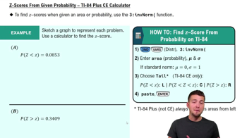
Z-Scores From Given Probability - TI-84 (CE) Calculator

Normal Quantile Plot

A normal quantile plot is a graphical tool used to assess if a dataset follows a normal distribution. It plots the z-scores of the data against the expected z-scores from a standard normal distribution. If the points on the plot form a roughly straight line, it suggests that the data are normally distributed; deviations from this line indicate departures from normality.
Recommended video:
04:01
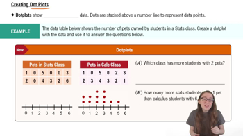
Creating Dotplots

Normal Distribution

Normal distribution is a probability distribution that is symmetric about the mean, showing that data near the mean are more frequent in occurrence than data far from the mean. It is characterized by its bell-shaped curve and is defined by two parameters: the mean and the standard deviation. Understanding normal distribution is crucial for interpreting the results of normal quantile plots and determining the likelihood of data belonging to a normal population.
Recommended video:
Guided course
09:47
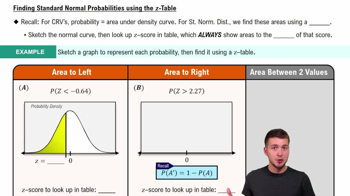
Finding Standard Normal Probabilities using z-Table
Related Practice
Textbook Question

Car Colors

In Exercises 9–12, assume that 100 cars are randomly selected. Refer to the accompanying graph, which shows the top car colors and the percentages of cars with those colors (based on PPG Industries).


Black Cars Find the probability that at least 25 cars are black. Is 25 a significantly high number of black cars?

125
views
Textbook Question

Outliers For the purposes of constructing modified boxplots as described in Section 3-3, outliers are defined as data values that are above Q3 by an amount greater than 1.5 x IQR or below Q1 by an amount greater than 1.5 x IQR, where IQR is the interquartile range. Using this definition of outliers, find the probability that when a value is randomly selected from a normal distribution, it is an outlier.

209
views
Textbook Question

Births: Sampling Distribution of Sample Proportion When two births are randomly selected, the sample space for genders is bb, bg, gb, and gg (where and Assume that those four outcomes are equally likely. Construct a table that describes the sampling distribution of the sample proportion of girls from two births. Does the mean of the sample proportions equal the proportion of girls in two births? Does the result suggest that a sample proportion is an unbiased estimator of a population proportion?

178
views
Textbook Question

Distributions In a continuous uniform distribution,


" style="" width="290">


a. Find the mean and standard deviation for the distribution of the waiting times represented in Figure 6-2, which accompanies Exercises 5–8.

246
views
Textbook Question

Standard Normal Distribution. In Exercises 17–36, assume that a randomly selected subject is given a bone density test. Those test scores are normally distributed with a mean of 0 and a standard deviation of 1. In each case, draw a graph, then find the probability of the given bone density test scores. If using technology instead of Table A-2, round answers to four decimal places.


Between 1.50 and 2.00

185
views
Textbook Question

Finding Bone Density Scores. In Exercises 37–40 assume that a randomly selected subject is given a bone density test. Bone density test scores are normally distributed with a mean of 0 and a standard deviation of 1. In each case, draw a graph, then find the bone density test score corresponding to the given information. Round results to two decimal places.


Find P99, the 99th percentile. This is the bone density score separating the bottom 99% from the top 1%.

184
views