
Ch. 9 - Differential Equations
Briggs - Calculus: Early Transcendentals 3rd Edition
Briggs3rd EditionCalculus: Early TranscendentalsISBN: 9780136847243Not the one you use?Change textbook
Chapter 9, Problem 9.R.32c

A first-order equation Consider the equation t² y′(t) + 2ty(t) = e⁻ᵗ
c. Find the solution that satisfies the condition y(1) = 0

Verified step by step guidance
1
Rewrite the given differential equation in standard linear form. The original equation is \(t^{2} y'(t) + 2t y(t) = e^{-t}\). Divide both sides by \(t^{2}\) (assuming \(t \neq 0\)) to get \(y'(t) + \frac{2}{t} y(t) = \frac{e^{-t}}{t^{2}}\).
Identify the integrating factor (IF) for the linear first-order ODE. The integrating factor is given by \(\mu(t) = e^{\int P(t) dt}\), where \(P(t) = \frac{2}{t}\). Calculate \(\mu(t) = e^{\int \frac{2}{t} dt} = e^{2 \ln |t|} = t^{2}\).
Multiply the entire differential equation by the integrating factor \(t^{2}\) to write the left side as a derivative of a product: \(t^{2} y'(t) + 2t y(t) = \frac{d}{dt} [t^{2} y(t)]\). So, the equation becomes \(\frac{d}{dt} [t^{2} y(t)] = e^{-t}\).
Integrate both sides with respect to \(t\): \(\int \frac{d}{dt} [t^{2} y(t)] dt = \int e^{-t} dt\). This gives \(t^{2} y(t) = -e^{-t} + C\), where \(C\) is the constant of integration.
Apply the initial condition \(y(1) = 0\) to find \(C\). Substitute \(t=1\) and \(y(1)=0\) into \(t^{2} y(t) = -e^{-t} + C\) to get \(1^{2} \cdot 0 = -e^{-1} + C\), which simplifies to \(C = e^{-1}\). Then express \(y(t)\) explicitly as \(y(t) = \frac{-e^{-t} + e^{-1}}{t^{2}}\).

Verified video answer for a similar problem:

This video solution was recommended by our tutors as helpful for the problem above.
Video duration:
4m
Was this helpful?

Key Concepts

Here are the essential concepts you must grasp in order to answer the question correctly.

First-Order Linear Differential Equations

A first-order linear differential equation has the form y' + p(t)y = q(t). Solving it involves finding an integrating factor to rewrite the equation in an exact derivative form, allowing integration to find the general solution.
Recommended video:
07:39
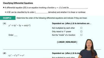
Classifying Differential Equations

Integrating Factor Method

The integrating factor is a function, usually denoted μ(t), used to multiply both sides of a linear differential equation to simplify it. It is typically μ(t) = e^(∫p(t) dt), which transforms the left side into the derivative of μ(t)y, facilitating integration.
Recommended video:
07:33
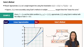
Euler's Method

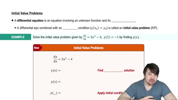
Initial Value Problems

An initial value problem specifies a condition like y(t₀) = y₀ to determine a unique solution from the general solution of a differential equation. Applying this condition allows solving for the constant of integration, yielding the particular solution.
Recommended video:
05:03
Initial Value Problems