Textbook Question
33–42. Solving initial value problems Solve the following initial value problems.
p'(x) = 2/(x² + x), p(1) = 0
48
views

 Verified step by step guidance
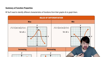
 06:21
06:21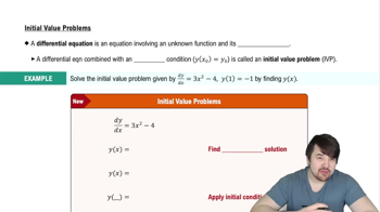 05:03
05:03 5:53
5:5333–42. Solving initial value problems Solve the following initial value problems.
p'(x) = 2/(x² + x), p(1) = 0
9–14. Growth rate functions Make a sketch of the population function P (as a function of time) that results from the following growth rate functions. Assume the population at time t = 0 begins at some positive value.
33–42. Solving initial value problems Solve the following initial value problems.
y''(t) = teᵗ, y(0) = 0, y'(0) = 1
45–46. Harvesting problems Consider the harvesting problem in Example 6.
If r = 0.05 and H = 500, for what values of p₀ is the amount of the resource decreasing? For what value of p₀ is the amount of the resource constant? If p₀ = 9000, when does the resource vanish?
11–16. Initial value problems Solve the following initial value problems.
y'(t) − 3y = 12, y(1) = 4
27–30. Newton’s Law of Cooling Solve the differential equation for Newton’s Law of Cooling to find the temperature function in the following cases. Then answer any additional questions.
An iron rod is removed from a blacksmith’s forge at a temperature of 900°C . Assume k=0.02 and the rod cools in a room with a temperature of 30°C When does the temperature of the rod reach 100°C?