
Textbook Question
Use the graph of the greatest integer function y = ⌊x⌋, Figure 1.10 in Section 1.1, to help you find the limits in Exercises 21 and 22.
<IMAGE>
b. limt→4−(t−⌊t⌋)
340
views
 Verified step by step guidance
 06:11
06:11
 05:18
05:18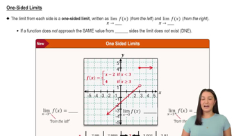 05:50
05:50Use the graph of the greatest integer function y = ⌊x⌋, Figure 1.10 in Section 1.1, to help you find the limits in Exercises 21 and 22.
<IMAGE>
b. limt→4−(t−⌊t⌋)
Average Rates of Change
In Exercises 1–6, find the average rate of change of the function over the given interval or intervals.
g(t)=2+cos t
b. [0,π]
Limits and Continuity
On what intervals are the following functions continuous?
b. g(x) = x³/⁴
Estimating Limits
[Technology Exercise] You will find a graphing calculator useful for Exercises 67–74.
Let f(x)=(x² − 1)/(|x| − 1).
b. Support your conclusion in part (a) by graphing f near c = -1 and using Zoom and Trace to estimate y-values on the graph as x→−1.
Exercises 5–10 refer to the function
f(x) = { x² − 1, −1 ≤ x < 0
2x, 0 < x < 1
1, x = 1
−2x + 4, 1 < x < 2
0, 2 < x < 3
graphed in the accompanying figure.
<IMAGE>
b. Does lim x → −1⁺ f (x) exist?
Estimating Limits
[Technology Exercise] You will find a graphing calculator useful for Exercises 67–74.
Let g(θ) = (sinθ) / θ.
b. Support your conclusion in part (a) by graphing g near θ₀ = 0.