Table of contents
- 0. Fundamental Concepts of Algebra3h 32m
- 1. Equations and Inequalities3h 27m
- 2. Graphs1h 43m
- 3. Functions & Graphs2h 17m
- 4. Polynomial Functions1h 54m
- 5. Rational Functions1h 23m
- 6. Exponential and Logarithmic Functions2h 28m
- 7. Measuring Angles40m
- 8. Trigonometric Functions on Right Triangles2h 5m
- 9. Unit Circle1h 19m
- 10. Graphing Trigonometric Functions1h 19m
- 11. Inverse Trigonometric Functions and Basic Trig Equations1h 41m
- 12. Trigonometric Identities 2h 34m
- 13. Non-Right Triangles1h 38m
- 14. Vectors2h 25m
- 15. Polar Equations2h 5m
- 16. Parametric Equations1h 6m
- 17. Graphing Complex Numbers1h 7m
- 18. Systems of Equations and Matrices3h 6m
- 19. Conic Sections2h 36m
- 20. Sequences, Series & Induction1h 15m
- 21. Combinatorics and Probability1h 45m
- 22. Limits & Continuity1h 49m
- 23. Intro to Derivatives & Area Under the Curve2h 9m
6. Exponential and Logarithmic Functions
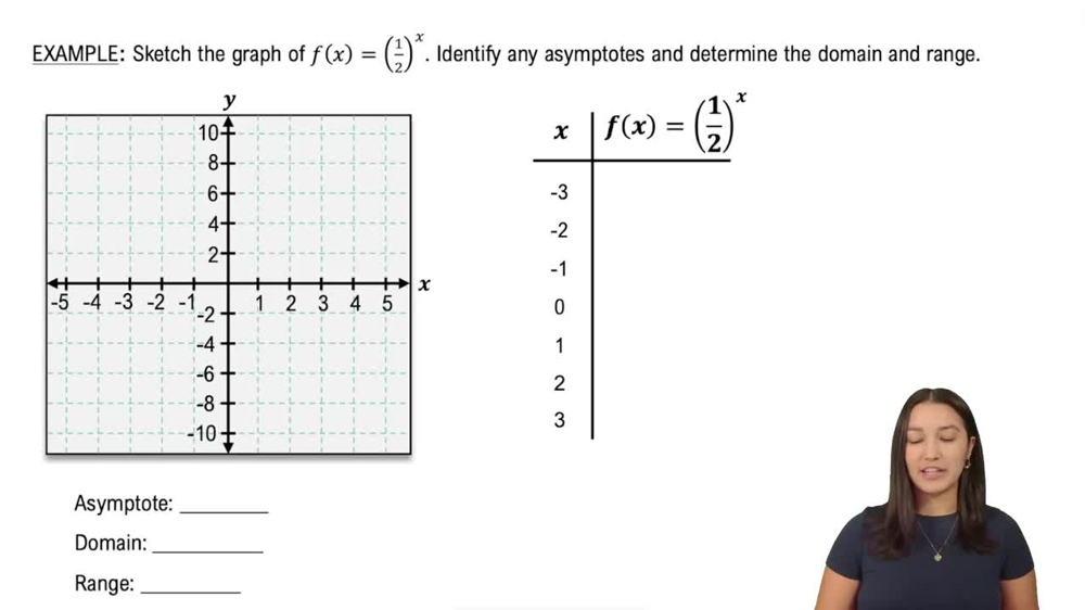
Graphing Exponential Functions


Graphs of Exponential Functions
Callie
Video duration:
5mPlay a video:
 3:58
3:58