Graphing Systems of Inequalities: Videos & Practice Problems

Graphing inequalities involves plotting corresponding lines or curves and shading regions that satisfy the inequality. For linear inequalities, a solid line indicates "greater than or equal to" or "less than or equal to," while a dashed line indicates "greater than" or "less than." Testing points helps determine which side to shade. Nonlinear inequalities, like quadratics, follow the same process. When dealing with multiple inequalities, the solution is found in the overlapping shaded regions, representing points that satisfy all inequalities simultaneously.

Linear Inequalities

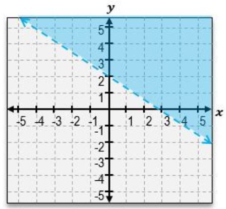
Graphing two-dimensional inequalities involves a few straightforward steps that build on the concepts of one-dimensional inequalities. When dealing with inequalities like \( x \geq 1 \), the first step is to graph the corresponding line, which in this case is a vertical line at \( x = 1 \). This line divides the plane into two regions. To determine which side to shade, you need to identify the points that satisfy the inequality. For example, testing the point \( (2, 0) \) shows that \( 2 \geq 1 \) is true, indicating that the region to the right of the line is where the inequality holds true.

When graphing inequalities with two variables, such as \( y < x \), you start by graphing the line \( y = x \). Since the inequality is strict (less than), you use a dashed line to indicate that points on the line are not included in the solution set. The next step is to determine which side of the line to shade. This can be done by testing a point not on the line, such as \( (0, 1) \). Plugging these coordinates into the inequality shows whether the point satisfies it. If it does, you shade the side of the line that includes that point.

For more complex inequalities like \( y > 2x - 4 \), the process remains similar. First, graph the line \( y = 2x - 4 \) using a dashed line since the inequality is strict. Then, test a point, such as \( (0, 1) \). If the point satisfies the inequality, shade the region that includes that point. In this case, since \( 1 > 2(0) - 4 \) simplifies to \( 1 > -4 \), which is true, you would shade the area above the line.

In summary, the key steps to graphing linear inequalities are: graph the corresponding line (solid for \( \geq \) or \( \leq \), dashed for \( > \) or \( < \)), test a point to see if it satisfies the inequality, and shade the appropriate region based on the result of the test. Additionally, if you can express the inequality in slope-intercept form, you can quickly determine that for \( y > mx + b \), you shade above the line, while for \( y < mx + b \), you shade below.

Example 1

In this exploration of systems of inequalities, we analyze three equations and their corresponding graphs. The first equation, y > -3x + 4, represents a line with a y-intercept of 4 and a slope of -3. To visualize this, we consider the line as if it were equal, which helps us identify the graph. Since the inequality is a greater than symbol, the line is dashed, indicating that the solution includes all points above the line. Thus, this equation corresponds to graph number 3.

Next, we examine the second equation, x + y < 1. To better understand its graph, we convert it to slope-intercept form: y < -x + 1. This line has a y-intercept of 1 and a slope of -1. The less than symbol indicates that the line is also dashed, and we shade below the line. This confirms that this equation matches graph number 2.

Finally, we look at the third equation, -3x - y ≥ -4. To simplify, we can multiply through by -1, which reverses the inequality, yielding 3x + y ≤ 4. Rewriting this in slope-intercept form gives us y ≤ -3x + 4. This line has the same y-intercept of 4 and a slope of -3 as the first equation, but the less than or equal to symbol indicates a solid line with shading below. Therefore, this equation corresponds to graph number 1.

In summary, we matched the equations to their graphs based on the characteristics of the lines and the direction of shading dictated by the inequality symbols. Understanding how to manipulate and interpret these inequalities is crucial for solving systems of inequalities effectively.

Graph the inequality $2x+3y$ < $6$.

• A.
• B.
• C.
• D.

Answer: (C)

Nonlinear Inequalities

Graphing nonlinear inequalities, such as quadratic equations, follows a similar process to graphing linear inequalities. For example, consider the inequality \( y \geq x^2 - 1 \). This represents a quadratic function, where the graph is a parabola. The first step is to determine whether to use a solid or dashed line based on the inequality symbol. Since the symbol is "greater than or equal to," a solid line will be used to indicate that points on the line are included in the solution set.

The equation \( y = x^2 - 1 \) has a vertex at the point (0, -1) and opens upwards. To visualize this, sketch the parabola, ensuring the vertex is correctly placed. Next, to determine which side of the parabola to shade, select a test point. A convenient choice is (0, 2), which lies above the parabola. Substitute these values into the inequality:

\( 2 \geq 0^2 - 1 \)

This simplifies to:

\( 2 \geq -1 \)

This statement is true, indicating that the region containing the point (0, 2) satisfies the inequality. Therefore, shade the area above the parabola, which represents all points where \( y \) is greater than or equal to \( x^2 - 1 \).

It is important to remember that the parabola acts as a boundary. While it may seem intuitive to shade everything above the curve, ensure that the shaded region is confined to the area that satisfies the inequality. Thus, the solution set includes all points above the parabola, effectively capturing the essence of the inequality.

In summary, graphing nonlinear inequalities involves determining the type of line to use, sketching the corresponding curve, testing points to identify the valid region, and shading appropriately to represent the solution set.

Graph the inequality $y$ < $2^{x}$.

• A.
• B.
• C.
• D.

Answer: (A)

Example 2

To graph the inequality \(x^2 + (y - 1)^2 \leq 9\), we start by determining the type of line to use. Since the inequality includes a "less than or equal to" symbol, we will use a solid line. This indicates that points on the boundary are included in the solution set.

Next, we rewrite the inequality as an equation to find the boundary: \(x^2 + (y - 1)^2 = 9\). This equation resembles the standard form of a circle, which is given by \((x - h)^2 + (y - k)^2 = r^2\), where \((h, k)\) is the center and \(r\) is the radius. In our case, the center of the circle is at \((0, 1)\) and the radius \(r\) can be found by taking the square root of 9, resulting in \(r = 3\).

To graph the circle, we plot the center at \((0, 1)\) and then move 3 units in all directions (up, down, left, and right) to mark the points \((0, 4)\), \((0, -2)\), \((3, 1)\), and \((-3, 1)\). Connecting these points will give us a circle with a solid line since the inequality includes the boundary.

After graphing the circle, we need to determine where to shade. To do this, we can test a point to see if it satisfies the inequality. A convenient point to test is \((2, 0)\). Substituting this point into the inequality gives:

\(2^2 + (0 - 1)^2 \leq 9\) which simplifies to \(4 + 1 \leq 9\) or \(5 \leq 9\). This statement is true, indicating that the area containing the point \((2, 0)\) is part of the solution set.

However, we must also check a point that is inside the circle but not on the boundary to ensure we are shading the correct area. Testing the point \((0, 0)\) yields:

\(0^2 + (0 - 1)^2 \leq 9\) simplifies to \(0 + 1 \leq 9\) or \(1 \leq 9\), which is also true. This confirms that the area inside the circle is part of the solution.

In conclusion, the solution to the inequality \(x^2 + (y - 1)^2 \leq 9\) is the region inside the circle, including the boundary. This method of testing points ensures that we accurately identify the area that satisfies the inequality.

Systems of Inequalities

Graphing a system of inequalities involves plotting multiple inequalities on the same coordinate plane and identifying the region where their shaded areas overlap. This overlapping region represents the solution set that satisfies all inequalities simultaneously.

To begin, each inequality is graphed individually. For instance, consider the inequality y ≤ -x + 4. This is represented by a solid line because the inequality includes equality (≤). The line intersects the y-axis at (0, 4) and has a slope of -1. After graphing the line, the area below it is shaded, indicating all points that satisfy this inequality.

Next, for the inequality y > 2x + 1, a dashed line is drawn since the inequality does not include equality (>). This line has a y-intercept of 1 and a slope of 2. The area above this line is shaded, representing the solutions to this inequality. Testing a point, such as (0, 2), confirms that it satisfies both inequalities, allowing for the appropriate shading.

After shading the regions for each inequality, the final step is to identify the overlapping area. This intersection is the solution to the system of inequalities, where all conditions are met. Different colors or shading styles can be used to distinguish between the inequalities, but the focus remains on the region where the shadings overlap.

In cases where one or more inequalities are nonlinear, such as parabolas, the same principles apply. For example, the inequality y ≥ x² - 4 represents a parabola opening upwards with a vertex at (0, -4). The area above this parabola is shaded, indicating the solutions. When combined with another linear inequality, the overlapping region will still represent the solution set.

It is also important to note that some systems of inequalities may have no solutions, which occurs when the shaded regions do not intersect at all. Understanding how to graph and analyze these inequalities is crucial for solving complex mathematical problems involving multiple conditions.

Graph the system of inequalities and indicate the region (if any) of solutions satisfying all equations.




$3x-2y>6$
$3x-2y$ < $-4$

• A.
• B.
• C.
• D.

Answer: (D)

Graph the system of inequalities and indicate the region (if any) of solutions satisfying all equations.


$x+y\le4$
$y\ge1$$x>0$

• A.
• B.
• C.
• D.

Answer: (B)

Here’s what students ask on this topic:

How do you graph a system of linear inequalities?

To graph a system of linear inequalities, follow these steps:

1. Graph each inequality separately by first plotting the corresponding line. Use a solid line for ≤ or ≥ and a dashed line for < or >.
2. Determine which side of the line to shade by testing a point not on the line. If the point satisfies the inequality, shade that side.
3. Repeat for all inequalities in the system.
4. The solution to the system is the region where the shaded areas overlap, representing points that satisfy all inequalities simultaneously.

What is the difference between a solid line and a dashed line when graphing inequalities?

A solid line is used when the inequality includes ≤ or ≥, indicating that points on the line are part of the solution set. A dashed line is used for < or >, indicating that points on the line are not included in the solution set. This visual distinction helps identify whether boundary points are included in the region that satisfies the inequality.

How do you determine which side of the line to shade when graphing an inequality?

To determine which side of the line to shade, select a test point not on the line (commonly the origin (0,0) if it is not on the line). Substitute the coordinates of the test point into the inequality. If the inequality holds true, shade the side of the line where the test point is located. If it does not hold true, shade the opposite side.

How do you graph nonlinear inequalities like quadratics?

Graphing nonlinear inequalities, such as quadratics, involves similar steps to linear inequalities:

1. Graph the corresponding equation (e.g., y = x² - 1) using a solid or dashed line based on the inequality symbol.
2. Determine which side of the curve to shade by testing a point not on the curve.
3. If the test point satisfies the inequality, shade the region that includes the point. Otherwise, shade the opposite region.
4. The shaded region represents the solution set for the inequality.

What happens if a system of inequalities has no solution?

If a system of inequalities has no solution, it means there is no region where the shaded areas of all inequalities overlap. This can occur if the inequalities represent regions that do not intersect. In such cases, the system is considered inconsistent, and there are no points that satisfy all inequalities simultaneously.