Graphing logarithmic functions can be straightforward, especially since they are the inverse of exponential functions. Understanding this relationship allows us to leverage our knowledge of exponential graphs to effectively graph logarithmic functions.
Consider the logarithmic function log2(x). To begin, we can generate ordered pairs by substituting values for x. For instance, when x = 1, we find that log2(1) = 0, giving us the point (1, 0). Similarly, for x = 2, log2(2) = 1, resulting in the point (2, 1). Notably, these points correspond to the points on the exponential function f(x) = 2x, specifically (0, 1) and (1, 2), but with the x and y values flipped due to their inverse relationship.
Continuing this process, we can derive additional points by flipping the coordinates of the exponential function. For example, the points (4, 2) and (8, 3) can be obtained by reflecting the points of the exponential function across the line y = x. This reflection is a key characteristic of inverse functions.
When graphing the logarithmic function, it is essential to note the presence of a vertical asymptote at x = 0, indicating that the graph approaches but never touches the y-axis. The overall shape of the logarithmic graph resembles an extended lowercase r, while the exponential graph resembles an extended lowercase e.
In terms of domain and range, the domain of the logarithmic function is all positive real numbers ((0, ∞)), while the range is all real numbers ((−∞, ∞)). This is a direct consequence of the properties of inverse functions, where the domain of the exponential function corresponds to the range of the logarithmic function and vice versa.
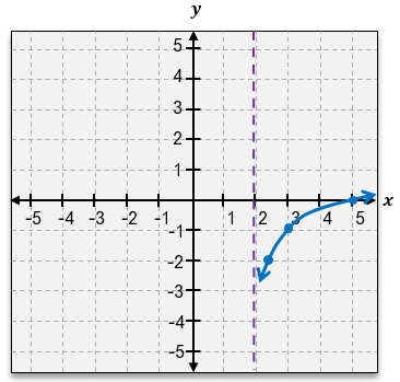
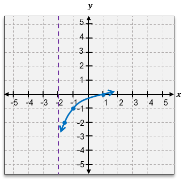
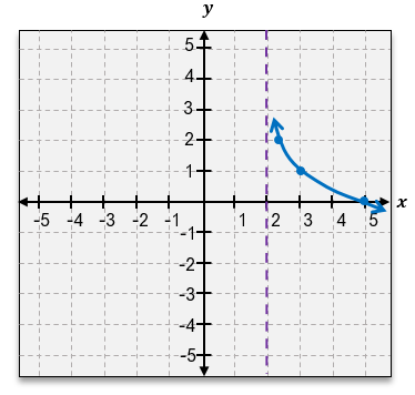
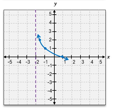
When considering logarithmic functions with different bases, the behavior of the graph remains consistent with that of exponential functions. If the base b is greater than 1, the logarithmic function will be increasing. Conversely, if b is between 0 and 1, the function will be decreasing. This relationship mirrors the behavior of exponential functions, reinforcing the connection between these two types of functions.
In summary, understanding the inverse relationship between logarithmic and exponential functions simplifies the process of graphing logarithmic functions. By utilizing known points from the exponential function and reflecting them, we can accurately depict the logarithmic graph while also considering its domain, range, and asymptotic behavior.