Slope Fields: Videos & Practice Problems

Slope fields, or direction fields, visualize solutions to first-order differential equations of the form $y\text{'}=f(x,\mathrm{y<mo>)</mo>}$. By sketching short line segments at each point on a coordinate system, we can determine slopes by substituting points into the derivative. This method reveals patterns that indicate the shape of solutions, allowing us to sketch particular solutions through given initial conditions, enhancing our understanding of differential equations.

Understanding Slope Fields

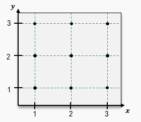
Differential equations are fundamental in understanding how functions change, and slope fields provide a visual representation of their solutions. A slope field, also known as a direction field, illustrates the slopes of solutions to a first-order differential equation of the form \( y' = f(x, y) \). By sketching short line segments at various points on a coordinate system, we can visualize the behavior of solutions even when we cannot explicitly solve the equation.

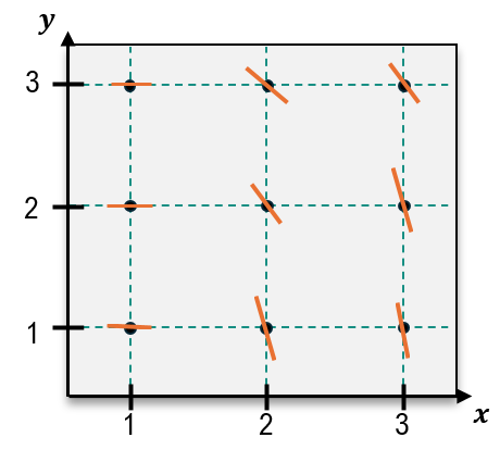
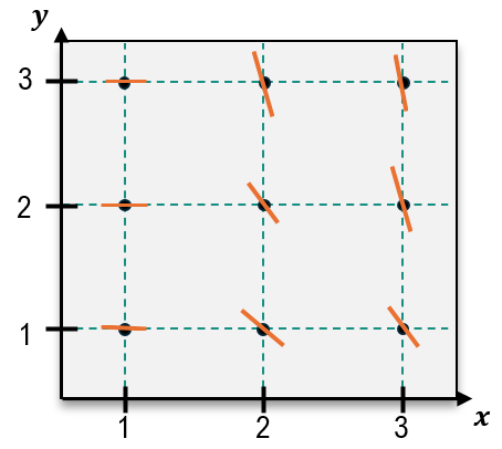
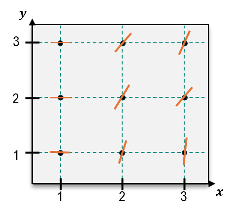
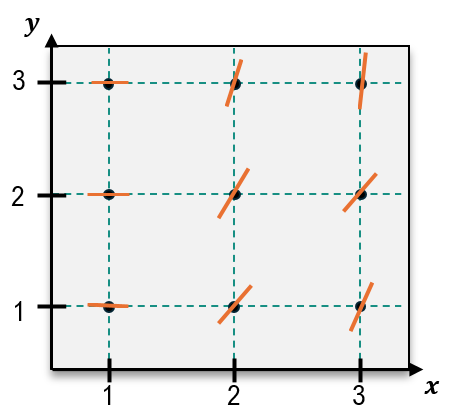
To create a slope field, we evaluate the derivative \( y' \) at specific points. For example, consider the differential equation \( y' = x - y \). To sketch the slope field, we calculate the slope at points like (1, 0), (1, 1), and (2, 0) by substituting these coordinates into the equation. For (1, 0), we find \( y' = 1 - 0 = 1 \), indicating a slope of 1. For (1, 1), \( y' = 1 - 1 = 0 \), resulting in a horizontal line segment. Continuing this process reveals patterns, such as zero slopes along the line where \( x = y \) and positive slopes along other diagonals.

Once the slope field is established, we can sketch particular solutions that pass through given initial conditions. For instance, to find the solution curve that passes through the point (-1, 2), we plot this point and follow the slopes indicated by the field. The curve will steepen and then curve back, potentially approaching a slant asymptote. This method can be repeated for any point, such as (1, -2), allowing us to visualize how solutions behave in relation to the slope field.

In summary, slope fields are a powerful tool for visualizing the solutions of differential equations, providing insight into their behavior without needing to solve them analytically. This approach enhances our understanding of the dynamics described by the equations and prepares us for further exploration of differential equations and their applications.

Understanding Slope Fields Example 1

In analyzing a slope field, each line segment corresponds to the slope of a function at a specific point defined by a differential equation. For instance, consider the differential equation $\frac{dy}{dx} = 3 - x$. If we evaluate this at the point (0,0), substituting 0 for x yields a slope of 3. However, the slope field does not exhibit a slope of 3 at this point, allowing us to eliminate this equation from consideration.

Next, we observe that at x = 0, the slope field shows no defined slopes, indicating that the derivative is undefined at this point. This observation helps us narrow down our options, as the other equations, including $\sin(2x)$ and $\frac{1}{2} \cos(x)$, remain defined at x = 0. This leads us to focus on the equation $\frac{dy}{dx} = \frac{1}{x}$, which is indeed undefined at x = 0.

Furthermore, as we analyze the slope field, we notice that as x increases, the slopes of the line segments become less steep. This behavior aligns with the characteristics of the equation $\frac{dy}{dx} = \frac{1}{x}$, where an increase in x results in a larger denominator, thus producing a smaller slope value. This trend is also observed in the negative direction, confirming the consistency of the slope field with this differential equation.

In conclusion, the differential equation represented by the given slope field is $\frac{dy}{dx} = \frac{1}{x}$, as it accurately reflects the observed patterns in the slope field.

Understanding Slope Fields Example 2

When analyzing slope fields and their corresponding differential equations, it's essential to identify patterns in the slopes that can help match them accurately. For the first slope field, a key observation is that along the line where \( x = 0 \), all line segments exhibit a zero slope. This indicates that any differential equation yielding a zero slope when \( x = 0 \) could be a candidate. The equation \( y' = x + y \) does not satisfy this condition since \( y \) can take on various values, resulting in non-zero slopes. However, the equation \( y' = 2x \) does yield a zero slope at \( x = 0 \), making it a strong contender. Additionally, as \( x \) increases, the slopes become steeper in both positive and negative directions, independent of \( y \). This reinforces that the correct match for this slope field is \( y' = 2x \).

Moving to the second slope field, a notable feature is the presence of diagonal lines where the slopes are zero at specific points, such as \( (-1, 1) \) and \( (2, -2) \). This suggests that the sum of \( x \) and \( y \) at these points results in a zero slope, aligning perfectly with the differential equation \( y' = x + y \). Further examination reveals that the slopes along the diagonal are consistently negative, confirming that this equation accurately represents the slope field.

In the final slope field, a circular pattern emerges, with zero slopes occurring when \( x = 0 \). This observation aligns with the remaining differential equation \( y' = -\frac{x}{y} \), as a zero numerator results in a zero slope. Additionally, the slopes are undefined along the line \( y = 0 \), which is consistent with the equation since \( y \) appears in the denominator. Thus, this differential equation matches the last slope field.

In summary, the slope fields correspond to the following differential equations: the first field matches \( y' = 2x \), the second field corresponds to \( y' = x + y \), and the final field aligns with \( y' = -\frac{x}{y} \). Understanding these relationships is crucial for solving differential equations and interpreting their graphical representations.

Understanding Slope Fields Example 3

To sketch a slope field for the differential equation \(\frac{dy}{dx} = y - 1\), we first recognize that the slopes depend solely on the value of \(y\). This means that for any given \(y\), the slope will be constant across the entire horizontal line at that \(y\) value. To visualize this, we can create a table of values for \(y\) and the corresponding slope, calculated as \(y - 1\).

For example:

• When \(y = 0\), the slope is \(0 - 1 = -1\).
• When \(y = 1\), the slope is \(1 - 1 = 0\).
• When \(y = 2\), the slope is \(2 - 1 = 1\).
• When \(y = 3\), the slope is \(3 - 1 = 2\).
• When \(y = -1\), the slope is \(-1 - 1 = -2\).
• When \(y = -2\), the slope is \(-2 - 1 = -3\).

From this table, we observe that as \(y\) increases, the slope becomes steeper, and similarly, it becomes steeper in the negative direction as \(y\) decreases. Specifically, at \(y = 1\), the slope is zero, indicating a horizontal line across the graph. This line acts as a horizontal asymptote for the solution curves.

Next, we can draw the slope field by plotting these slopes across the graph. For each \(y\) value, we draw a line segment with the corresponding slope. For instance, at \(y = 2\), we draw a line with a slope of 1 across the graph, and at \(y = 0\), we draw a line with a slope of -1. This process continues for all values of \(y\), creating a complete slope field.

Now, to sketch the particular solution curve through the initial condition \((-1, 0)\), we first plot the point \((-1, 0)\) on the graph. Following the slope field, we observe that as we move left from this point, the slope is negative, indicating that the curve will slope downward. As we approach the horizontal asymptote at \(y = 1\), the curve will get closer to this line but will never touch it, reflecting the behavior of the solution as it approaches the asymptote. Conversely, as we move downward from the initial point, the curve will steepen, reflecting the increasing negative slope.

In summary, the slope field provides a visual representation of the behavior of the solutions to the differential equation, while the particular solution curve illustrates how the function behaves given the initial condition. This understanding is crucial for analyzing the dynamics of differential equations and their solutions.

Sketch a slope field for the following differential equation through the nine points shown on the graph. 
$y^{\prime}=y-xy$

• A.
• B.
• C.
• D.

Answer: (B)

Here’s what students ask on this topic:

What is a slope field and how is it used in solving differential equations?

A slope field, also known as a direction field, is a graphical representation of the solutions to a first-order differential equation of the form $y^{\text{'}}=f(x,y)$. It consists of short line segments drawn at various points on a coordinate system, where the slope of each segment is determined by substituting the coordinates of the point into the derivative. Slope fields help visualize the behavior of solutions to differential equations, even when explicit solutions are not available. By observing patterns in the slope field, we can sketch particular solution curves that pass through given initial conditions, enhancing our understanding of the equation's dynamics.

How do you construct a slope field for a given differential equation?

To construct a slope field for a differential equation like $y^{\text{'}}=f(x,y)$, follow these steps: 1) Choose a grid of points on the coordinate system. 2) For each point, substitute its coordinates into the derivative $f(x,y)$ to calculate the slope. 3) Draw a short line segment at each point with the calculated slope. Repeat this process for all points in the grid. The resulting slope field will reveal patterns that indicate the shape of solutions to the differential equation.

How can slope fields help visualize particular solutions to differential equations?

Slope fields help visualize particular solutions by providing a graphical representation of the slopes at various points. To sketch a particular solution, start at the given initial condition (a specific point on the graph) and follow the slopes indicated by the field. The solution curve will pass through the initial condition and align with the direction of the slopes. This method allows us to approximate the behavior of the solution without solving the differential equation explicitly, making it a valuable tool for understanding complex equations.

What are the steps to sketch a particular solution using a slope field?

To sketch a particular solution using a slope field: 1) Identify the initial condition, which is a specific point on the graph. 2) Plot this point on the slope field. 3) Starting from the initial condition, follow the direction of the slopes indicated by the field. Draw the curve smoothly, ensuring it aligns with the slope segments at each point. 4) Continue tracing the curve in both directions until the desired range is covered. This process provides an approximation of the solution curve that passes through the given initial condition.

What patterns can be observed in slope fields, and how do they relate to differential equations?

Slope fields often reveal patterns such as regions of constant slope, symmetry, or diagonal lines where slopes are zero. These patterns correspond to specific behaviors of the differential equation. For example, if $y^{\text{'}}=x-y$, points where $x=y$ will have zero slope, forming a diagonal line. Observing these patterns helps us understand the general behavior of solutions and identify key features like equilibrium points or asymptotes.