Table of contents
- 0. Basic Principles of Economics1h 5m
- Introduction to Economics3m
- People Are Rational2m
- People Respond to Incentives1m
- Scarcity and Choice2m
- Marginal Analysis9m
- Allocative Efficiency, Productive Efficiency, and Equality7m
- Positive and Normative Analysis7m
- Microeconomics vs. Macroeconomics2m
- Factors of Production5m
- Circular Flow Diagram5m
- Graphing Review10m
- Percentage and Decimal Review4m
- Fractions Review2m
- 1. Reading and Understanding Graphs59m
- 2. Introductory Economic Models1h 10m
- 3. The Market Forces of Supply and Demand2h 26m
- Competitive Markets10m
- The Demand Curve13m
- Shifts in the Demand Curve24m
- Movement Along a Demand Curve5m
- The Supply Curve9m
- Shifts in the Supply Curve22m
- Movement Along a Supply Curve3m
- Market Equilibrium8m
- Using the Supply and Demand Curves to Find Equilibrium3m
- Effects of Surplus3m
- Effects of Shortage2m
- Supply and Demand: Quantitative Analysis40m
- 4. Elasticity2h 26m
- Percentage Change and Price Elasticity of Demand19m
- Elasticity and the Midpoint Method20m
- Price Elasticity of Demand on a Graph11m
- Determinants of Price Elasticity of Demand6m
- Total Revenue Test13m
- Total Revenue Along a Linear Demand Curve14m
- Income Elasticity of Demand23m
- Cross-Price Elasticity of Demand11m
- Price Elasticity of Supply12m
- Price Elasticity of Supply on a Graph3m
- Elasticity Summary9m
- 5. Consumer and Producer Surplus; Price Ceilings and Floors3h 45m
- Consumer Surplus and Willingness to Pay38m
- Producer Surplus and Willingness to Sell26m
- Economic Surplus and Efficiency18m
- Quantitative Analysis of Consumer and Producer Surplus at Equilibrium28m
- Price Ceilings, Price Floors, and Black Markets38m
- Quantitative Analysis of Price Ceilings and Price Floors: Finding Points20m
- Quantitative Analysis of Price Ceilings and Price Floors: Finding Areas54m
- 6. Introduction to Taxes and Subsidies1h 46m
- 7. Externalities1h 12m
- 8. The Types of Goods1h 13m
- 9. International Trade1h 16m
- 10. The Costs of Production2h 35m
- 11. Perfect Competition2h 24m
- Introduction to the Four Market Models2m
- Characteristics of Perfect Competition6m
- Revenue in Perfect Competition14m
- Perfect Competition Profit on the Graph20m
- Short Run Shutdown Decision34m
- Long Run Entry and Exit Decision18m
- Individual Supply Curve in the Short Run and Long Run6m
- Market Supply Curve in the Short Run and Long Run9m
- Long Run Equilibrium12m
- Perfect Competition and Efficiency15m
- Four Market Model Summary: Perfect Competition5m
- 12. Monopoly2h 13m
- Characteristics of Monopoly21m
- Monopoly Revenue12m
- Monopoly Profit on the Graph16m
- Monopoly Efficiency and Deadweight Loss20m
- Price Discrimination22m
- Antitrust Laws and Government Regulation of Monopolies11m
- Mergers and the Herfindahl-Hirschman Index (HHI)17m
- Four Firm Concentration Ratio6m
- Four Market Model Summary: Monopoly4m
- 13. Monopolistic Competition1h 9m
- 14. Oligopoly1h 26m
- 15. Markets for the Factors of Production1h 26m
- 16. Income Inequality and Poverty36m
- 17. Asymmetric Information, Voting, and Public Choice39m
- 18. Consumer Choice and Behavioral Economics1h 16m
11. Perfect Competition
Market Supply Curve in the Short Run and Long Run


Market Supply Curve in the Long Run
Brian Krogol
Video duration:
6mPlay a video:
Related Videos
Related Practice
 06:02
06:02