Use of Tech Linear and quadratic approximation


a. Find the linear approximating polynomial for the following functions centered at the given point a.


b. Find the quadratic approximating polynomial for the following functions centered at a.


c Use the polynomials obtained in parts (a) and (b) to approximate the given quantity.


Find the Taylor polynomials p₁, …, p₅ centered at a=0 for f(x)=e⁻ˣ

Verified step by step guidance

1. Step 1: Understand the problem requires finding Taylor polynomials of degrees 1 through 5 for the function \(f(x) = e^{-x}\) centered at \(a=0\). Recall that the Taylor polynomial of degree \(n\) centered at \(a\) is given by: \[p_n(x) = \sum_{k=0}^n \frac{f^{(k)}(a)}{k!} (x - a)^k\] where \(f^{(k)}(a)\) is the \(k\)-th derivative of \(f\) evaluated at \(a\).
2. Step 2: Compute the derivatives of \(f(x) = e^{-x}\) up to the 5th order. Note the pattern in derivatives: - \(f(x) = e^{-x}\) - \(f'(x) = -e^{-x}\) - \(f''(x) = e^{-x}\) - \(f^{(3)}(x) = -e^{-x}\) - \(f^{(4)}(x) = e^{-x}\) - \(f^{(5)}(x) = -e^{-x}\) This alternating pattern will help in evaluating derivatives at \(x=0\).
3. Step 3: Evaluate each derivative at \(a=0\). Since \(e^0 = 1\), the values will alternate between \(1\) and \(-1\) depending on the order of the derivative: - \(f(0) = 1\) - \(f'(0) = -1\) - \(f''(0) = 1\) - \(f^{(3)}(0) = -1\) - \(f^{(4)}(0) = 1\) - \(f^{(5)}(0) = -1\)
4. Step 4: Write the Taylor polynomials \(p_1\) through \(p_5\) by substituting the derivative values into the Taylor polynomial formula: \[p_n(x) = \sum_{k=0}^n \frac{f^{(k)}(0)}{k!} x^k\] For example, the linear polynomial \(p_1(x)\) includes terms up to \(k=1\), the quadratic \(p_2(x)\) up to \(k=2\), and so on.
5. Step 5: Use the polynomials \(p_1\) and \(p_2\) (linear and quadratic approximations) to approximate values of \(f(x)\) near \(x=0\) by plugging in the desired \(x\) values into these polynomials. This provides an approximation of \(e^{-x}\) using simpler polynomial expressions.

Key Concepts

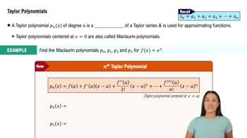
Taylor Polynomials

Taylor polynomials approximate a function near a point by using its derivatives at that point. The nth-degree Taylor polynomial is constructed from the function's value and its first n derivatives evaluated at the center, providing increasingly accurate approximations as n increases.

Linear and Quadratic Approximations

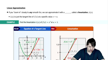
Linear approximation uses the first-degree Taylor polynomial (tangent line) to estimate function values near a point, while quadratic approximation uses the second-degree polynomial, incorporating curvature via the second derivative. These approximations simplify complex functions for easier calculation.

Evaluating and Using Taylor Polynomials for Approximation

Once Taylor polynomials are found, they can be used to approximate function values at points near the center. This involves substituting the desired x-value into the polynomial, providing a practical method to estimate values without computing the original function directly.