Consider the differential equation y'(t) = t² - 3y² and the solution curve that passes through the point (3, 1). What is the slope of the curve at (3, 1)?
Table of contents
- 0. Functions7h 54m
- Introduction to Functions16m
- Piecewise Functions10m
- Properties of Functions9m
- Common Functions1h 8m
- Transformations5m
- Combining Functions27m
- Exponent rules32m
- Exponential Functions28m
- Logarithmic Functions24m
- Properties of Logarithms36m
- Exponential & Logarithmic Equations35m
- Introduction to Trigonometric Functions38m
- Graphs of Trigonometric Functions44m
- Trigonometric Identities47m
- Inverse Trigonometric Functions48m
- 1. Limits and Continuity2h 2m
- 2. Intro to Derivatives1h 33m
- 3. Techniques of Differentiation3h 18m
- 4. Applications of Derivatives2h 38m
- 5. Graphical Applications of Derivatives6h 2m
- 6. Derivatives of Inverse, Exponential, & Logarithmic Functions2h 37m
- 7. Antiderivatives & Indefinite Integrals1h 26m
- 8. Definite Integrals4h 44m
- 9. Graphical Applications of Integrals2h 27m
- 10. Physics Applications of Integrals 3h 16m
- 11. Integrals of Inverse, Exponential, & Logarithmic Functions2h 34m
- 12. Techniques of Integration7h 41m
- 13. Intro to Differential Equations2h 55m
- 14. Sequences & Series5h 36m
- 15. Power Series2h 19m
- 16. Parametric Equations & Polar Coordinates7h 58m
13. Intro to Differential Equations
Basics of Differential Equations
Problem 9.R.28b
Textbook Question
Logistic growth in India The population of India was 435 million in 1960 (t=0) and 487 million in 1965 (t=5). The projected population for 2050 is 1.57 billion.
b. Use the solution of the logistic equation and the 2050 projected population to determine the carrying capacity.
Verified step by step guidance1
Recall the general form of the logistic growth model: \[ P(t) = \frac{K}{1 + Ae^{-rt}} \] where \(P(t)\) is the population at time \(t\), \(K\) is the carrying capacity, \(r\) is the growth rate, and \(A\) is a constant related to initial conditions.
Use the initial condition at \(t=0\) (year 1960) where \(P(0) = 435\) million to express \(A\) in terms of \(K\): \[ 435 = \frac{K}{1 + A} \implies A = \frac{K}{435} - 1 \]
Use the population at \(t=5\) (year 1965), \(P(5) = 487\) million, and substitute \(A\) into the logistic equation: \[ 487 = \frac{K}{1 + \left(\frac{K}{435} - 1\right) e^{-5r}} \] This equation relates \(K\) and \(r\).
Use the projected population for 2050, which corresponds to \(t=90\) (since 2050 - 1960 = 90), where \(P(90) = 1570\) million (1.57 billion). Substitute into the logistic model: \[ 1570 = \frac{K}{1 + \left(\frac{K}{435} - 1\right) e^{-90r}} \]
Now you have two equations involving \(K\) and \(r\) from steps 3 and 4. Solve this system of equations simultaneously to find the carrying capacity \(K\).
Verified video answer for a similar problem:
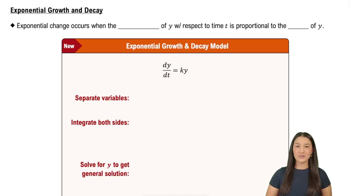
This video solution was recommended by our tutors as helpful for the problem above
Video duration:
2mPlay a video:
Was this helpful?
Key Concepts
Here are the essential concepts you must grasp in order to answer the question correctly.
Logistic Growth Model
The logistic growth model describes population growth that starts exponentially but slows as it approaches a maximum limit called the carrying capacity. It is represented by a differential equation where growth rate decreases as population nears this limit, modeling realistic constraints like resources.
Recommended video:
Exponential Growth & Decay
Carrying Capacity
Carrying capacity is the maximum population size that an environment can sustain indefinitely given available resources. In the logistic model, it is the horizontal asymptote that the population approaches over time, representing the stable equilibrium point.
Recommended video:
Intro to the Chain Rule Example 2
Using Logistic Equation Solutions to Estimate Parameters
Solving the logistic differential equation yields a formula for population over time involving parameters like growth rate and carrying capacity. By substituting known population values at specific times, one can solve for unknown parameters such as the carrying capacity.
Recommended video:
Guided course
Eliminate Parameter: Equations with Trig
Watch next
Master Classifying Differential Equations with a bite sized video explanation from Patrick
Start learningRelated Videos
Related Practice
Textbook Question
13
views
