Residuals: Videos & Practice Problems

Linear regression utilizes the least squares method to find the line of best fit, minimizing residuals, which are the vertical distances from data points to the regression line. Residuals are calculated as $d=y-\mathrm{ŷ}$, where y is the observed value and ŷ is the predicted value. A residual plot helps assess the fit; random patterns indicate a good fit, while discernible patterns suggest a poor fit, necessitating alternative models. Understanding these concepts is crucial for effective data analysis and predictive modeling.

Residuals and Residual Plots

Linear regression is a statistical method used to model the relationship between a dependent variable and one or more independent variables. The least squares method is a common technique employed to find the line of best fit, which minimizes the sum of the squared residuals. A residual is defined as the vertical distance between an observed data point and the predicted value on the regression line, represented mathematically as:

$$d = y - \hat{y}$$

where \(d\) is the residual, \(y\) is the actual observed value, and \(\hat{y}\) is the predicted value from the regression equation.

To calculate residuals, one must first determine the predicted values (\(\hat{y}\)) using the regression equation. For example, if the regression equation is given as:

$$\hat{y} = 284x - 16101$$

then for a specific \(x\) value, you substitute \(x\) into the equation to find \(\hat{y}\). The residual is then calculated by subtracting the predicted value from the actual value. Residuals can be positive or negative, indicating whether the actual value is above or below the predicted value.

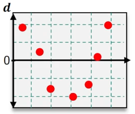
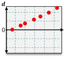
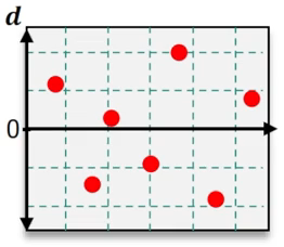
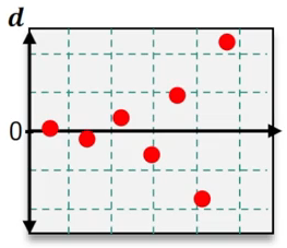
Once all residuals are calculated, they can be visualized using a residual plot, where the x-axis represents the original data values and the y-axis represents the residuals. This plot helps assess the fit of the regression model. A good fit is indicated by a random scatter of residuals around the horizontal axis, suggesting no discernible pattern. Conversely, if the residuals display a systematic pattern, such as oscillation or divergence, it indicates that the linear model may not be appropriate for the data.

In summary, analyzing residuals and their plots is crucial for evaluating the effectiveness of a linear regression model. A random distribution of residuals supports the model's validity, while patterns in the residuals suggest the need for alternative modeling approaches.

Which of the following residual plots suggest that a linear regression model is appropriate?

• A.
• B.
• C.
• D.

Answer: (C)

Here’s what students ask on this topic:

What is a residual in linear regression?

A residual in linear regression is the vertical distance between an observed data point and the predicted value on the regression line. It represents the error or difference between the actual value ($y$) and the predicted value ($y_{^}$) calculated using the regression equation. Mathematically, it is expressed as:

$d=y-y_{^}$

Residuals help assess how well the regression line fits the data. Smaller residuals indicate a better fit, while larger residuals suggest the model may not capture the data's variability effectively. Residuals can be positive or negative, depending on whether the observed value is above or below the predicted value.

How do you calculate residuals in a dataset?

To calculate residuals in a dataset, follow these steps:

1. Use the regression equation to calculate the predicted value ($y_{^}$) for each $x$ value in the dataset.
2. Subtract the predicted value from the observed value ($y$) for each data point. The formula is:

$d=y-y_{^}$

For example, if the observed value is 10 and the predicted value is 8, the residual is:

$d=\; 10\; -\; 8\; =\; 2$

Repeat this process for all data points in the dataset to calculate their respective residuals.

What is a residual plot, and how is it used?

A residual plot is a graph that displays residuals ($d$) on the y-axis and the corresponding independent variable ($x$) on the x-axis. It helps assess the fit of a regression model by visualizing the distribution of residuals.

If the residuals are randomly scattered around the horizontal axis (y = 0), it indicates that the regression model is a good fit for the data. However, if the residuals show a discernible pattern (e.g., oscillation or divergence), it suggests that the model may not adequately capture the relationship, and a different model might be needed.

Residual plots are essential for diagnosing issues like non-linearity, heteroscedasticity (non-constant variance), or outliers in the data.

What does it mean if residuals show a pattern in a residual plot?

If residuals show a pattern in a residual plot, it indicates that the regression model may not be a good fit for the data. Common patterns include:

• Oscillation: Residuals alternate in a wave-like pattern, suggesting a non-linear relationship that a linear model cannot capture.
• Divergence: Residuals spread out as $x$ increases, indicating heteroscedasticity (non-constant variance).

Such patterns suggest that the assumptions of linear regression (e.g., linearity, constant variance) are violated. In these cases, alternative models, such as polynomial regression or transformations, may be more appropriate.

Why are residuals important in regression analysis?

Residuals are important in regression analysis because they measure the accuracy of the model's predictions. By analyzing residuals, you can:

• Assess the goodness of fit: Smaller residuals indicate a better fit, while larger residuals suggest the model may not capture the data's variability effectively.
• Diagnose model issues: Patterns in residuals can reveal problems like non-linearity, heteroscedasticity, or outliers.
• Validate assumptions: Randomly scattered residuals confirm that the linear regression assumptions (e.g., linearity, constant variance) are met.

Residual analysis is a critical step in ensuring the reliability and validity of a regression model.