Quadratic Regression: Videos & Practice Problems

Quadratic regression models data with a curve using the equation $y=a{x}^2+bx+c$, where $a$ controls curvature. Using a TI-84 calculator, input data into lists, select quadratic regression, and store the equation as $y$₁ for graphing. The coefficient of determination ($R^2$) near 1 indicates a strong fit, essential for predictive analytics and regression analysis. This method aids in modeling nonlinear trends, enhancing data mining and statistical process control accuracy.

Quadratic Regression Using TI-84

Quadratic regression is a powerful statistical method used to model data that follows a curved pattern rather than a straight line. Unlike linear regression, which fits data to a line defined by the equation y = bx + c, quadratic regression fits data to a parabola described by the equation
\[ y = ax^2 + bx + c \]
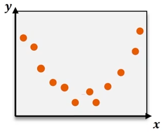
where the ax² term introduces the curvature, allowing the model to capture U-shaped or inverted U-shaped trends in the data.

When analyzing datasets that exhibit nonlinear behavior, such as sales trends over time that rise and then fall, quadratic regression provides a more accurate fit. The coefficients a, b, and c represent the parameters of the quadratic equation, with a controlling the curvature, b the linear component, and c the y-intercept.

To determine these coefficients efficiently, graphing calculators like the TI-84 offer built-in quadratic regression functions. By entering the data points into lists (commonly L1 for x-values and L2 for y-values), users can access the quadratic regression feature through the statistics menu. The calculator computes the best-fit quadratic equation by minimizing the sum of squared residuals, providing values for a, b, and c automatically.

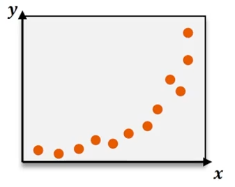
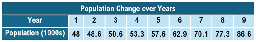
For example, analyzing toy sales over nine weeks might yield a quadratic regression equation such as:
\[ \hat{y} = -2.07x^2 + 20.63x - 1.05 \]
where the negative coefficient of x² indicates a concave downward curve, reflecting sales that increase and then decrease over time.

Evaluating the goodness of fit is crucial, and this is often done using the coefficient of determination, R². This statistic ranges from 0 to 1, with values closer to 1 indicating a better fit. An R² value of 0.977, for instance, suggests that the quadratic model explains approximately 97.7% of the variance in the data, confirming the model’s accuracy.

After calculating the regression equation, graphing it alongside the original data points helps visualize the fit. Adjusting the graph window to encompass the range of x-values and y-values ensures the curve and data points are clearly displayed. Activating the scatter plot feature on the calculator allows the data points to be plotted, while the stored regression equation (often saved as Y1) can be graphed simultaneously, illustrating how well the quadratic curve aligns with the data.

In summary, quadratic regression extends linear regression by incorporating a squared term to model curved data trends effectively. Utilizing graphing calculators streamlines the process of finding the best-fit quadratic equation and assessing its fit through the R² value. This method is especially useful in real-world scenarios where relationships between variables are nonlinear, enabling more accurate predictions and insights.

For the data points in the graphs below, which most likely suggests a quadratic relationship?

• A.
• B.
• C.
• D.

Answer: (C)

The data below shows the population of a small town (in 1000s) over a 9 year period. Using a graphing calculator, determine the linear & quadratic regression curves. Compare their $R^2$ values. Which model is a better fit for the data?

• A. Both Linear with $R^2=0.93$ and quadratic with $R^2=0.999$ are good fits for the data.
• B. Quadratic with $R^2=0.999$ is a better fit than linear with with $R^2=0.96$.
• C. Both Linear with $R^2=0.96$ and quadratic with $R^2=0.999$ are good fits for the data.
• D. Quadratic with $R^2=0.999$ is a better fit than linear with with $R^2=0.93$.

Answer: (D)

Quadratic Regression Using TI-84 Example 1

In analyzing production costs, quadratic regression is a powerful tool to model the relationship between the number of units produced and the average cost per unit. By inputting production data into a graphing calculator, such as the TI-84, one can determine the quadratic regression equation that best fits the data. This equation typically takes the form:

$$y\; =\; ax^2\; +\; bx\; +\; c$$

where y represents the average cost per unit, x is the number of units produced, and a, b, and c are coefficients derived from the regression analysis. For example, a quadratic regression might yield coefficients such as a = 0.0052, b = -0.61, and c = 26.73, resulting in the equation:

$$y\; =\; 0.0052x^2\; -\; 0.61x\; +\; 26.73$$

The quality of this model is assessed using the coefficient of determination, denoted as R². An R² value close to 1 indicates a strong fit between the model and the observed data. In practical terms, an R² value above 0.8 is considered a good fit, suggesting the quadratic model accurately captures the cost behavior across production runs.

Using this quadratic regression equation, predictions can be made for production levels beyond the original data set. For instance, to estimate the average cost per unit when producing 100 units, substitute x = 100 into the equation:

$$y\; =\; 0.0052(100)^2\; -\; 0.61(100)\; +\; 26.73$$

Calculating this yields an average cost of approximately \$17.73 per unit at 100 units produced. This prediction reveals an important insight: the average cost per unit decreases initially, reaching a minimum at around 60 units, and then begins to increase as production continues to rise. This behavior reflects the quadratic nature of the cost function, where economies of scale reduce costs up to a point, after which factors such as increased labor or overhead cause costs to climb again.

From a business perspective, this analysis informs decision-making regarding production levels. Since the average cost per unit at 100 units is significantly higher than at 60 units, it may not be economically advantageous for the plant to increase output beyond the point where costs are minimized. Understanding this cost optimization helps managers balance production volume with cost efficiency, ultimately supporting more profitable operations.

Here’s what students ask on this topic:

What is quadratic regression and how does it differ from linear regression?

Quadratic regression is a statistical method used to model data that follows a curved pattern rather than a straight line. Unlike linear regression, which fits data to a line using the equation $y=bx+c$, quadratic regression fits data to a parabola using the equation $y=a{x}^2+bx+c$. The key difference is the $a{x}^2$ term, which allows the curve to bend upward or downward, capturing nonlinear trends in the data. This makes quadratic regression ideal for datasets where the relationship between variables is not a straight line but a curve, such as U-shaped or inverted U-shaped patterns.

How do you perform quadratic regression using a TI-84 graphing calculator?

To perform quadratic regression on a TI-84 calculator, first enter your data into lists by pressing STAT > EDIT and inputting your x-values into L1 and y-values into L2. Next, press STAT > CALC and select the quadratic regression option (usually 5: QuadReg). Enter L1, L2 for the x and y lists, and optionally store the regression equation to Y1 by pressing VARS > Y-VARS > Function > Y1. After calculating, the calculator will display coefficients $a$, $b$, and $c$ for the equation $y=a{x}^2+bx+c$. You can then graph the curve by pressing GRAPH with the plot turned on.

What does the coefficient of determination (R²) tell us in quadratic regression?

The coefficient of determination, denoted as $R^2$, measures how well the quadratic regression model fits the data. It ranges from 0 to 1, where values closer to 1 indicate a better fit. For example, an $R^2$ value of 0.977 means that approximately 97.7% of the variation in the dependent variable is explained by the quadratic model. In practical terms, a high $R^2$ suggests the quadratic curve closely follows the data points, making it reliable for predictions. Generally, an $R^2$ above 0.8 is considered a strong fit in regression analysis.

When should you use quadratic regression instead of linear regression?

You should use quadratic regression when your data shows a curved pattern rather than a straight line. If the scatterplot of your data points forms a U-shape or an inverted U-shape, this indicates a nonlinear relationship that linear regression cannot accurately model. Quadratic regression, with its $a{x}^2$ term, captures this curvature effectively. Using quadratic regression in such cases improves the accuracy of predictions and better represents the underlying relationship between variables. If the data appears linear, then linear regression is sufficient.

How do you interpret the coefficients in a quadratic regression equation?

In a quadratic regression equation $y=a{x}^2+bx+c$, each coefficient has a specific role. The coefficient $a$ controls the curvature of the parabola; if $a$ is positive, the curve opens upward (U-shaped), and if negative, it opens downward (inverted U). The coefficient $b$ affects the slope and direction of the curve, influencing where the vertex (maximum or minimum point) occurs. The constant $c$ represents the y-intercept, or the value of $y$ when $x$ is zero. Together, these coefficients define the shape and position of the quadratic curve fitting the data.