Two-Way ANOVA: Videos & Practice Problems

Two-way ANOVA analyzes the effects of two factors on a dependent variable, testing for interaction effects where one factor's impact depends on the other. Hypotheses involve null and alternative statements for interaction and individual factors. The F-statistic, a ratio of mean squares, determines significance via p-values compared to an alpha level. Interaction plots visually assess interaction by plotting response variables against one factor, with lines representing the other; non-parallel lines indicate interaction. This method complements ANOVA tables, enhancing understanding of factor independence and combined effects in experimental design and statistical inference.

Intro to Two-Way ANOVA & Two-Way Tables

Two-way ANOVA is a statistical method used to compare the means of a dependent variable across two different factors simultaneously. Unlike one-way ANOVA, which examines differences across one factor, two-way ANOVA evaluates how two independent variables influence the outcome and whether there is an interaction effect between them. For example, in studying plant growth, factors such as sunlight exposure (low, medium, high) and fertilizer level (one tablespoon, three tablespoons) can both impact growth, and two-way ANOVA helps analyze these effects together.

In two-way ANOVA, the dependent variable is measured across all combinations of the two factors, often arranged in a data table with one factor along the rows and the other along the columns. The analysis involves testing three hypotheses: first, whether there is an interaction effect between the two factors; second, whether the first factor alone has a significant effect; and third, whether the second factor alone has a significant effect.

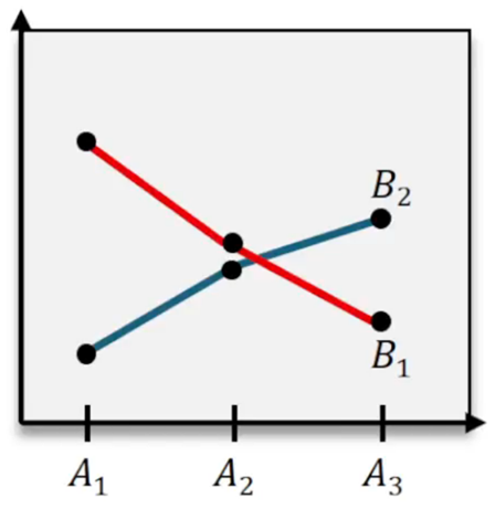
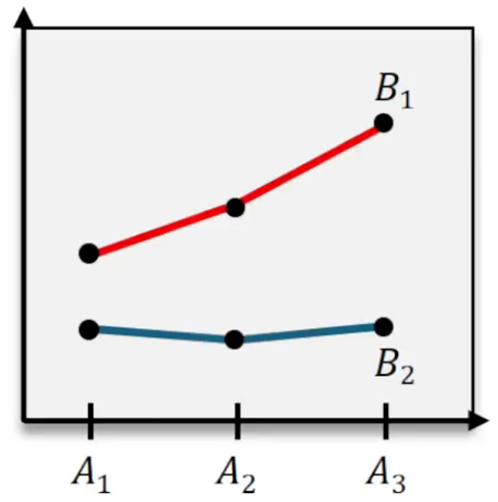
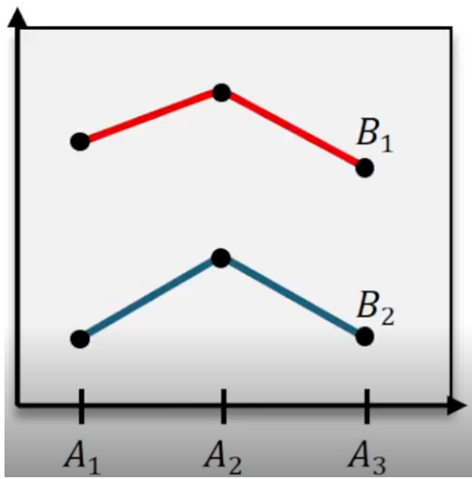
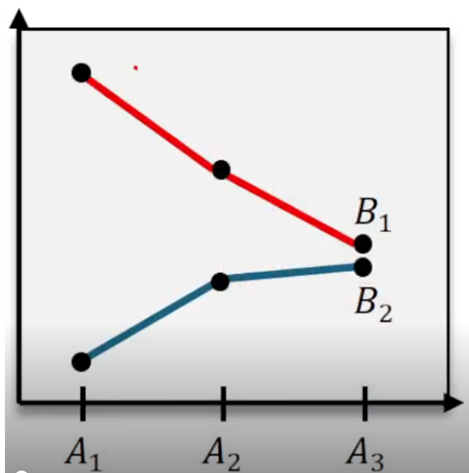
An interaction effect occurs when the effect of one factor on the dependent variable depends on the level of the other factor. For instance, if increasing fertilizer leads to a small increase in plant growth under low sunlight but a much larger increase under high sunlight, this indicates an interaction between fertilizer and sunlight. Detecting interaction is crucial because if a significant interaction exists, it complicates the interpretation of the individual effects of each factor.

The hypotheses for the interaction effect are set as follows: the null hypothesis (\(H_0\)) states that there is no interaction between the factors, while the alternative hypothesis (\(H_a\)) claims that an interaction exists. To test this, the F statistic is calculated as the ratio of the mean square due to interaction (\(MS_{\text{interaction}}\)) to the mean square error (\(MS_{\text{error}}\)):

\[F = \frac{MS_{\text{interaction}}}{MS_{\text{error}}}\]

The resulting F value is then used to find a p-value, which is compared to a significance level (commonly \(\alpha = 0.05\)). If the p-value is greater than \(\alpha\), we fail to reject the null hypothesis, indicating no significant interaction. This allows us to proceed with testing the main effects of each factor independently.

For the main effects, the hypotheses are similar: the null hypothesis assumes no difference in means across the levels of the factor, and the alternative hypothesis assumes a difference exists. The F statistic for each factor is calculated by dividing the mean square of that factor (\(MS_{\text{factor}}\)) by the mean square error:

\[F = \frac{MS_{\text{factor}}}{MS_{\text{error}}}\]

A p-value less than \(\alpha\) leads to rejecting the null hypothesis, providing evidence that the factor significantly affects the dependent variable. For example, if increasing fertilizer levels yields a very small p-value (e.g., 0.0001), it suggests a significant increase in plant growth with more fertilizer. Similarly, a significant effect of sunlight exposure indicates that varying sunlight levels also influence growth.

In summary, two-way ANOVA allows for a comprehensive analysis of how two factors and their potential interaction affect a dependent variable. By first testing for interaction effects and then examining the main effects, researchers can accurately interpret complex data where multiple variables influence outcomes. This method is widely applicable in experimental designs involving multiple categorical independent variables and continuous dependent variables.

Which of the following scenarios can be appropriately answered using a Two-Way ANOVA test?

• A. Researchers compare final exam scores between students who attended tutoring vs. who did not
• B. A psychologist compares anxiety levels among patients receiving one of two treatments
• C. A nutritionist studies how meal type (breakfast, lunch, dinner) and diet plan (low-carb, low-fat, Mediterranean) affect blood sugar levels
• D. A professor tests if average scores on a quiz are significantly different between 5 class sections

Answer: (C)

A university surveys how study group size (solo, duo, group) and study environment (quiet, noisy) affect test performance. Which of the following conclusions most clearly suggests an interaction effect between the two factors?

• A. Students who study in quiet environments score higher than students who study in noisy ones, regardless of group size
• B. Students who study in groups generally perform better than those who study alone, regardless of environment
• C. Solo and group sizes produced similar, higher scores overall, but duo group sizes were overall lower
• D. Students studying in groups in noisy environments tend to perform better, whereas students studying solo in quiet environments tend to perform better

Answer: (D)

Intro to Two-Way ANOVA & Two-Way Tables Example 1

In analyzing the effects of two factors—machine type (Type A vs. Type B) and operator experience (novice, intermediate, expert)—on the average number of defective units produced, a two-way ANOVA is used to determine if there are significant differences or interactions between these factors. The response variable in this context is the number of defective units produced per month.

The primary focus in a two-way ANOVA is to first test for an interaction effect between the two factors. An interaction effect occurs when the influence of one factor depends on the level of the other factor. The null hypothesis for the interaction effect states that there is no interaction between machine type and operator experience, while the alternative hypothesis suggests that an interaction does exist.

To test this, the p-value associated with the interaction term is compared to the significance level, typically set at α = 0.05. If the p-value is less than α, the null hypothesis is rejected, indicating evidence of an interaction effect. In this case, the p-value for the interaction was 0.027, which is less than 0.05, leading to the conclusion that there is a statistically significant interaction between machine type and operator experience affecting the number of defective units.

When an interaction effect is present, it implies that the effect of one factor cannot be fully understood without considering the other factor. Therefore, it is generally inappropriate to interpret the main effects independently. However, if required, the main effects can still be examined with caution. For the main effects, the p-values for machine type and operator experience were 0.052 and 0.556, respectively. Since both p-values exceed the 0.05 threshold, the null hypotheses for these main effects are not rejected, indicating no significant individual effect of machine type or operator experience alone on the defective units.

In summary, the presence of a significant interaction effect suggests that the combination of machine type and operator experience influences the defect rate in a way that cannot be explained by either factor alone. This highlights the importance of considering interaction effects in factorial experiments to avoid misleading conclusions about the individual factors.

Two-Way ANOVA: Interaction Plots

In analyzing the effects of two factors on a dependent variable, an interaction plot provides a visual method to detect interaction effects without complex calculations. When studying how factors such as hours of sleep and study time influence student performance on a nationwide exam, the interaction plot helps illustrate whether the impact of one factor depends on the level of the other.

To construct an interaction plot, the dependent variable—in this case, exam scores—is plotted on the y-axis, while one of the factors, such as hours of sleep, is placed on the x-axis. The second factor, study time, is represented by separate lines on the graph, each corresponding to different categories (e.g., low and high study time). Points are plotted for each combination of factor levels, and these points are connected with line segments to visualize trends.

The key to interpreting interaction plots lies in the comparison of these line segments. If the lines are approximately parallel, it suggests no interaction effect, meaning the effect of one factor on the dependent variable is consistent regardless of the level of the other factor. Conversely, if the lines are not parallel and show different slopes or shapes—such as crossing or diverging—this indicates an interaction effect. This means the influence of one factor varies depending on the level of the other factor.

For example, if exam scores increase with more hours of sleep for both low and high study time groups, but the increase is much steeper for the high study time group, the lines will not be parallel. This non-parallelism suggests that the combined effect of sleep and study time on exam performance is not simply additive but interactive.

While interaction plots provide a straightforward visual tool to hypothesize about interaction effects, statistical tests like two-way ANOVA are necessary to confirm these effects with significance. Nonetheless, understanding how to create and interpret interaction plots is essential for exploring complex relationships between multiple factors in experimental data.

Which of the following interaction plots best indicates no interaction between the two factors?

• A.
• B.
• C.
• D.

Answer: (C)

Here’s what students ask on this topic:

What is the main purpose of conducting a two-way ANOVA in statistical analysis?

Two-way ANOVA is used to analyze the effects of two independent factors on a dependent variable simultaneously. It helps determine not only the individual impact of each factor but also whether there is an interaction effect between them. An interaction effect occurs when the effect of one factor depends on the level of the other factor. This method extends one-way ANOVA by allowing researchers to understand complex relationships in experimental designs, such as how different levels of sunlight and fertilizer affect plant growth. By testing hypotheses using F-statistics and p-values, two-way ANOVA provides a comprehensive view of how multiple factors and their combinations influence outcomes.

How do you interpret the interaction effect in a two-way ANOVA?

In two-way ANOVA, the interaction effect tests whether the influence of one factor on the dependent variable changes depending on the level of the other factor. If the interaction is significant (p-value < alpha), it means the factors do not act independently, and the effect of one factor varies with the other. For example, fertilizer might increase plant growth more under high sunlight than low sunlight. If the interaction is not significant, the factors are considered independent, and their effects can be interpreted separately. Testing for interaction is crucial because a significant interaction can affect how you interpret the main effects of each factor.

What is an interaction plot and how does it help in understanding two-way ANOVA results?

An interaction plot is a graphical tool used to visualize the relationship between two factors and their effect on a dependent variable. In the plot, one factor is placed on the x-axis, the dependent variable on the y-axis, and lines represent different levels of the second factor. If the lines are roughly parallel, it suggests no interaction effect, meaning the factors act independently. If the lines cross or diverge, it indicates an interaction effect, where the effect of one factor depends on the other. Interaction plots provide a quick, visual way to assess potential interactions before conducting formal statistical tests.

What are the null and alternative hypotheses when testing for interaction effects in two-way ANOVA?

When testing for interaction effects in two-way ANOVA, the null hypothesis ($H{0}_{}$) states that there is no interaction between the two factors, meaning the effect of one factor does not depend on the level of the other. The alternative hypothesis ($H{a}_{}$) states that there is an interaction effect, meaning the factors influence the dependent variable jointly. Formally, $H{0}_{}:\; ext\{No\; interaction\; effect\}$ and $H{a}_{}$: ext{Interaction effect exists}. The decision to reject or fail to reject $H{0}_{}$ is based on the F-statistic and corresponding p-value compared to the significance level.

How do you calculate the F-statistic for each factor and interaction in a two-way ANOVA?

In two-way ANOVA, the F-statistic for each factor and the interaction is calculated as the ratio of the mean square (MS) for that factor or interaction to the mean square error (MSE). Mathematically, for a factor or interaction, the F-statistic is $\frac{{\mathrm{MS}}_{\mathrm{factor}}}{{\mathrm{MS}}_{\mathrm{error}}}$. Here, ${\mathrm{MS}}_{\mathrm{factor}}$ is the mean square due to the factor or interaction, and ${\mathrm{MS}}_{\mathrm{error}}$ is the mean square due to error (within-group variability). This ratio measures how much variation is explained by the factor relative to random error. A larger F-statistic suggests a significant effect, which is then tested against a critical value or p-value at a chosen alpha level.

What steps should be followed when analyzing two-way ANOVA results?

When analyzing two-way ANOVA results, first test for the interaction effect between the two factors. If the interaction is significant, interpret the interaction and avoid interpreting main effects separately because the factors influence each other. If the interaction is not significant, proceed to test the main effects of each factor independently. For each test, state the null and alternative hypotheses, calculate the F-statistic, and compare the p-value to the significance level (usually 0.05). Finally, interpret the results: reject the null hypothesis if p < 0.05, indicating a significant effect, or fail to reject if p >= 0.05, indicating no significant effect. This approach ensures accurate conclusions about factor effects and their interactions.