Find the exact length of the curve given by , for .
Table of contents
- 0. Functions7h 55m
- Introduction to Functions18m
- Piecewise Functions10m
- Properties of Functions9m
- Common Functions1h 8m
- Transformations5m
- Combining Functions27m
- Exponent rules32m
- Exponential Functions28m
- Logarithmic Functions24m
- Properties of Logarithms36m
- Exponential & Logarithmic Equations35m
- Introduction to Trigonometric Functions38m
- Graphs of Trigonometric Functions44m
- Trigonometric Identities47m
- Inverse Trigonometric Functions48m
- 1. Limits and Continuity2h 2m
- 2. Intro to Derivatives1h 33m
- 3. Techniques of Differentiation3h 18m
- 4. Applications of Derivatives2h 38m
- 5. Graphical Applications of Derivatives6h 2m
- 6. Derivatives of Inverse, Exponential, & Logarithmic Functions2h 37m
- 7. Antiderivatives & Indefinite Integrals1h 26m
- 8. Definite Integrals4h 44m
- 9. Graphical Applications of Integrals2h 27m
- 10. Physics Applications of Integrals 3h 16m
- 11. Integrals of Inverse, Exponential, & Logarithmic Functions2h 31m
- 12. Techniques of Integration7h 41m
- 13. Intro to Differential Equations2h 55m
- 14. Sequences & Series5h 36m
- 15. Power Series2h 19m
- 16. Parametric Equations & Polar Coordinates7h 58m
1. Limits and Continuity
Finding Limits Algebraically
Problem 9.1.53d
Textbook Question
52-56. In this section, several models are presented and the solution of the associated differential equation is given. Later in the chapter, we present methods for solving these differential equations.
where P(t) is the population, for t ≥ 0, and r > 0 and K > 0 are given constants.
d. Find lim(t→∞) P(t) and check that the result is consistent with the graph in part (c).
 Verified step by step guidance
1
Identify the differential equation model given for the population \(P(t)\), which is typically the logistic growth model: \[\frac{dP}{dt} = rP\left(1 - \frac{P}{K}\right),\] where \(r > 0\) is the growth rate and \(K > 0\) is the carrying capacity.
Understand that the equilibrium solutions occur when the growth rate is zero, i.e., when \[\frac{dP}{dt} = 0.\] This happens if either \(P = 0\) or \(P = K\).
Analyze the stability of these equilibrium points: since \(r > 0\), \(P = 0\) is an unstable equilibrium and \(P = K\) is a stable equilibrium, meaning the population tends to \(K\) as \(t \to \infty\).
Therefore, to find \[\lim_{t \to \infty} P(t),\] recognize that the solution \(P(t)\) approaches the stable equilibrium \(K\) over time.
Finally, verify that this limit is consistent with the graph in part (c), which should show the population leveling off at the carrying capacity \(K\) as time increases.
 Verified video answer for a similar problem:
This video solution was recommended by our tutors as helpful for the problem above
Video duration:
2mPlay a video:
0 Comments
Key Concepts
Here are the essential concepts you must grasp in order to answer the question correctly.
Logistic Differential Equation
The logistic differential equation models population growth with a carrying capacity, expressed as dP/dt = rP(1 - P/K). Here, P(t) is the population at time t, r is the growth rate, and K is the maximum sustainable population. Understanding this equation helps analyze how populations grow and stabilize over time.
Recommended video:

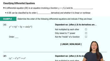
Classifying Differential Equations
Limit of a Function as t Approaches Infinity
The limit lim(t→∞) P(t) describes the long-term behavior of the population. Evaluating this limit reveals the steady-state or equilibrium population size. In logistic growth, this limit typically equals the carrying capacity K, indicating population stabilization.
Recommended video:

Limits of Rational Functions: Denominator = 0
Equilibrium Solutions and Stability
Equilibrium solutions occur when the population does not change over time (dP/dt = 0). For the logistic model, P = 0 and P = K are equilibria. Stability analysis shows that P = K is stable, meaning the population tends to this value as t increases, consistent with the graph's behavior.
Recommended video:

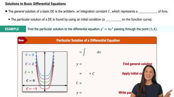
Solutions to Basic Differential Equations

 5:21m
5:21mWatch next
Master Finding Limits by Direct Substitution with a bite sized video explanation from Patrick
Start learningRelated Videos
Related Practice
Multiple Choice
28
views
