Linear Inequalities in One Variable: Videos & Practice Problems

Linear inequalities, expressed as $\mathrm{ax}+b>c$ or with other inequality symbols, have solutions represented by ranges rather than single values. These solutions can be depicted using set builder notation, interval notation, or number lines, with parentheses or brackets indicating inclusion or exclusion of boundary points. Solving inequalities involves isolating the variable using addition, subtraction, multiplication, or division, similar to linear equations. However, multiplying or dividing by a negative number requires flipping the inequality symbol to maintain a true statement, ensuring accurate solutions in algebraic expressions.

Introduction to Linear Inequalities

Linear inequalities are closely related to linear equations but differ by replacing the equal sign with an inequality symbol such as >, <, ≥, or ≤. A linear inequality takes the form \(ax + b > c\), \(ax + b < c\), \(ax + b \geq c\), or \(ax + b \leq c\), where \(a\), \(b\), and \(c\) are constants and \(x\) is the variable. This contrasts with a linear equation, which is typically written as \(ax + b = c\).

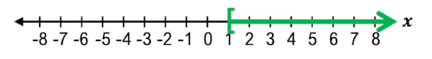
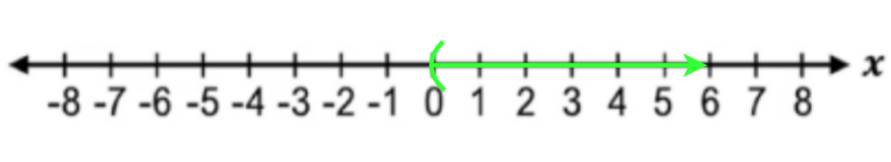
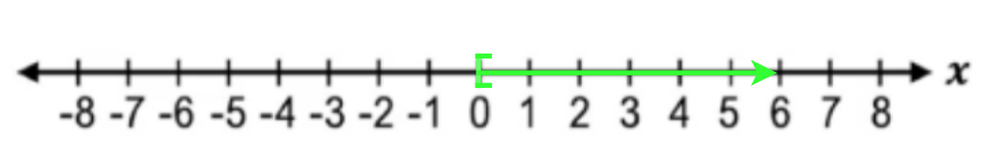
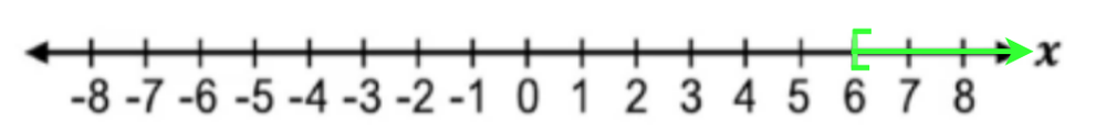
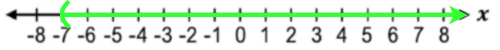
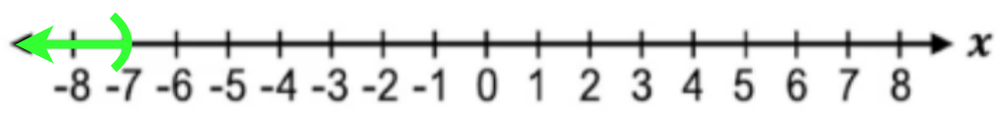
The solution to a linear inequality is the set of all values of \(x\) that make the inequality true when substituted back into the expression. Unlike linear equations, which usually have a single solution, linear inequalities often have a range of solutions. For example, solving the inequality \$2x - 6 > 0\( leads to \)x > 3\(, meaning any value greater than 3 satisfies the inequality.

To verify solutions, you can substitute values from the solution set back into the inequality. For instance, plugging in \)x = 5\( into \)2x - 6 > 0\( yields \)2(5) - 6 = 10 - 6 = 4\(, and since \)4 > 0\( is true, \)x = 5$ is indeed a valid solution. This process confirms that the solution to a linear inequality is not just a single number but an entire range of values that satisfy the inequality condition.

Understanding linear inequalities is fundamental for solving and graphing inequalities, as well as for interpreting solution sets in real-world contexts. The methods for solving linear inequalities build upon the techniques used for linear equations, with additional attention to the direction of the inequality and the range of solutions. This foundational knowledge prepares you to explore various representations of inequality solutions, including interval notation and graphical solutions on number lines.

Representing Solutions to Linear Inequalities

When solving inequalities, the solution is not a single value but a range of values. Understanding how to represent and visualize these solution sets is essential. One common way to express inequalities is through set builder notation. For example, the inequality x > 3 can be written as { x | x > 3 }, which reads as "the set of x such that x is greater than 3." The vertical bar "|" means "such that," and the curly brackets enclose the entire solution set.

Another way to visualize inequalities is on a number line. For x > 3, you start at 3 and draw an arrow pointing to the right, indicating all values greater than 3. Since 3 itself is not included, this is shown by using a parenthesis or an open circle at 3, symbolizing exclusion.

Interval notation offers a concise way to represent these ranges. For x > 3, the interval is written as (3, \infty). Parentheses indicate that 3 is not included, and infinity always uses parentheses because it is not a finite value and cannot be included.

When the inequality includes equality, such as x ≥ 3, the notations adjust accordingly. In set builder notation, it becomes { x | x ≥ 3 }. On the number line, the point at 3 is included, represented by a closed circle or a square bracket. In interval notation, this is written as [3, \infty), where the square bracket shows inclusion of 3, and the parenthesis at infinity remains.

For inequalities where x < 3 or x ≤ 3, the same principles apply but in the opposite direction. The number line arrow points left, and interval notation uses negative infinity. For example, x < 3 is (-\infty, 3) and x ≤ 3 is (-\infty, 3]. Parentheses indicate exclusion, and square brackets indicate inclusion of the endpoint.

It is important to remember that infinity and negative infinity are never included in intervals, so they always use parentheses. Additionally, on graphs, open circles denote excluded endpoints, while closed circles denote included endpoints. Although parentheses and square brackets are more commonly used in interval notation, recognizing open and closed circles on number lines is helpful for interpreting inequalities visually.

Mastering these notations—set builder, number line, and interval notation—enables clear communication and understanding of solution sets for linear inequalities, which is foundational for solving and graphing inequalities effectively.

Which inequality matches the graph?

• A. $x\ge1$
• B. $x\le1$
• C. $x>1$
• D. $x<1$

Answer: (A)

Which inequality matches the graph?

• A. $x\ge1$
• B. $x\le1$
• C. $x>1$
• D. $x<1$

Answer: (D)

Use the number line to graph the following inequality.

$x\ge 6$

• A.
• B.
• C.
• D.

Answer: (C)

Use the number line to graph the following inequality.

$x\ge -7$

• A.
• B.
• C.
• D.

Answer: (A)

Write the following in interval notation.
$x\ge 0$

• A. $\left(-\infty,0\right)$
• B. $\left\lbrack0,\infty\right)$
• C. $\left(0,\infty\right)$
• D. $\left(-\infty,0\right\rbrack$

Answer: (B)

Write the following in interval notation.

• A. $\left(-\infty,7\right\rbrack$
• B. $\left\lbrack7,\infty\right)$
• C. $\left(7,\infty\right)$
• D. $\left(-\infty,7\right)$

Answer: (D)

Rewrite the following as an inequality statement.
$(-\infty ,2]$

• A. $x\le2$
• B. $x<2$
• C. $x\ge2$
• D. $x>2$

Answer: (A)

Rewrite the following as an inequality statement.
$(1,\infty )$

• A. $x\ge1$
• B. $x\le1$
• C. $x>1$
• D. $x<1$

Answer: (C)

Introduction to Linear Inequalities Example 1

Understanding how to translate between inequalities, interval notation, and graphical representations is essential for mastering the concept of inequalities. When given an inequality such as x > -2, it corresponds to the interval notation (-2, ∞), where the parenthesis indicates that -2 is not included in the set. This matches a graph starting just after -2 and extending infinitely to the right.

For inequalities that include the boundary value, such as x ≥ -5, the interval notation uses a square bracket to denote inclusion: [-5, ∞). This means the set includes -5 and all values greater than -5, which is reflected in the graph by a solid point at -5 and an arrow extending to infinity.

Intervals like (4, ∞) represent values greater than 4 but not including 4 itself, indicated by a parenthesis. The corresponding graph starts just after 4 and extends to the right, without including the point at 4.

When dealing with values less than a number, such as values less than -2, the interval notation is (-∞, -2), where the parenthesis again shows that -2 is not included. The graph for this interval starts from negative infinity and ends just before -2.

Intervals that include the endpoint, like (-∞, 3], represent all values less than or equal to 3. The square bracket at 3 indicates inclusion, and the graph reflects this with a solid point at 3 and an arrow extending to the left towards negative infinity.

It is important to recognize that inequalities can be written in different forms but represent the same set. For example, -1 ≤ x is equivalent to x ≥ -1. This inequality corresponds to the interval [-1, ∞) and a graph starting at -1 (included) and extending to infinity.

By carefully analyzing the inequality symbols, interval notation, and graph characteristics—such as whether endpoints are included (square brackets) or excluded (parentheses)—one can accurately match these different representations. This skill enhances comprehension of how inequalities describe ranges of values and how these ranges are visually and symbolically expressed.

Solving Linear Inequalities

Solving linear inequalities involves isolating the variable using properties similar to those applied in linear equations, but with attention to the inequality symbols. The addition and subtraction properties of inequalities state that if A is greater than B, then adding or subtracting the same value C to both sides preserves the inequality: \(A + C > B + C\) and \(A - C > B - C\). For example, to solve \(x - 3 > 11\), add 3 to both sides to isolate x, resulting in \(x > 14\).

Multiplication and division properties also apply, where multiplying or dividing both sides of an inequality by a positive number maintains the inequality's direction. For instance, if \$2 < \frac{x}{5}\(, multiplying both sides by 5 yields \)10 < x\(. However, a critical distinction arises when multiplying or dividing by a negative number: the inequality symbol must be reversed to maintain a true statement. This is because multiplying or dividing by a negative value changes the sign of each side, necessitating flipping the inequality symbol.

For example, solving \)-7x \geq 21\( requires dividing both sides by \)-7\(. Since \)-7\( is negative, the inequality flips from \)\geq\( to \)\leq\(, giving \)x \leq -3$. This rule ensures the solution remains valid and highlights the importance of carefully handling inequalities involving negative multiplication or division.

In summary, solving linear inequalities involves isolating the variable using addition, subtraction, multiplication, and division, just like linear equations. The key difference is that when multiplying or dividing by a negative number, the inequality symbol must be reversed. Mastery of these properties allows for accurate solutions to linear inequalities, a fundamental skill in algebra.

Solving Linear Inequalities Example 2

To solve the linear inequality x + 8 ≤ 12 - x, start by gathering all variable terms on one side and constants on the other. Add x to both sides to eliminate the negative x on the right, resulting in 2x + 8 ≤ 12. Next, subtract 8 from both sides to isolate the variable term: 2x ≤ 4. Finally, divide both sides by 2 to solve for x, giving x ≤ 2.

Graphing this solution on a number line involves marking the point at 2 and shading all values less than or equal to 2. Since the inequality includes equality, use a closed circle or square bracket at 2 to indicate that 2 is part of the solution set.

Expressed in interval notation, the solution is (-∞, 2]. Parentheses are used with infinity because infinity is not a number and cannot be included, while the square bracket at 2 shows that 2 is included in the interval.

This process demonstrates how to solve linear inequalities by applying inverse operations, similar to solving linear equations, while paying attention to inequality symbols to correctly represent the solution set both graphically and in interval notation.

Solve the following linear inequalities using the addition and subtraction properties of equality.

• A. $x<2$
• B. $x>2$
• C. $x<1.8$
• D. $x\le1.8$

Answer: (A)

Solve the following linear inequalities and write the solution in interval notation.
$2(x+4)\le 3(x-1)+x$

• A. $\frac{11}{2}\ge x$
• B. $\frac{11}{2}\le x$
• C. $\frac{11}{4}\le x$
• D. $\frac{11}{4}\ge x$

Answer: (B)

Solve the following linear inequalities and write the solution in interval notation.

• A. $x<-\frac52$
• B. $x<-\frac{18}{5}$
• C. $x>-\frac{18}{5}$
• D. $x>-\frac52$

Answer: (C)

Solving Linear Inequalities Example 3

When solving inequalities, it is important to isolate the variable terms on one side and the constants on the other. For example, consider the inequality \$2x - 5 < 2x + 10\(. By subtracting \)2x\( from both sides, the variable terms cancel out, leaving \)-5 < 10\(. Since this statement is always true, the solution to the inequality is all real numbers. This means that no matter what value of \)x\( is substituted, the inequality holds true. Such inequalities are similar to identity equations in algebra, where the solution set includes every real number.

In contrast, consider the inequality \)x + 2 \geq x + 8\(. Subtracting \)x\( from both sides results in \)2 \geq 8\(, which is a false statement. This indicates that the inequality has no solution, as there is no value of \)x$ that can satisfy it. This type of inequality is called inconsistent, analogous to contradiction equations in linear algebra, where no solution exists.

Understanding these outcomes helps in recognizing when inequalities represent all real numbers, no solution, or a specific range of values. The process of solving inequalities involves careful manipulation of terms and interpreting the resulting statements to determine the solution set. This foundational skill is essential for solving more complex algebraic inequalities and understanding their graphical representations on the number line.

Here’s what students ask on this topic:

What is a linear inequality and how does it differ from a linear equation?

A linear inequality is similar to a linear equation but instead of an equal sign, it uses inequality symbols such as >, <, ≥, or ≤. For example, a linear equation looks like $\mathrm{2x}-6=0$, while a linear inequality might be $\mathrm{2x}-6>0$. The key difference is that the solution to a linear equation is a single value of $x$ that satisfies the equation, whereas the solution to a linear inequality is a range of values that make the inequality true. For example, $x>3$ means any value greater than 3 satisfies the inequality, not just one specific number.

How do you represent the solution of a linear inequality using interval notation?

Interval notation is a concise way to represent the solution set of a linear inequality. For example, if the solution is $x>3$, the interval notation is $(3,\; 21)$, where the parenthesis around 3 means 3 is not included, and infinity (21) always has a parenthesis because it is not a real number and cannot be included. If the inequality is $x253$ (less than or equal to 3), the interval notation is $(-21,\; 3]$, where the square bracket means 3 is included in the solution set. Parentheses indicate exclusion of endpoints, while square brackets indicate inclusion.

What is the rule for solving linear inequalities when multiplying or dividing by a negative number?

When solving linear inequalities, if you multiply or divide both sides of the inequality by a negative number, you must reverse the direction of the inequality symbol. For example, if you have $-7x\; 25\; 21$ and divide both sides by $-7$, the inequality flips from $25$ to $24$, resulting in $x\; 24\; -3$. This rule is essential because multiplying or dividing by a negative number changes the order of the values, so flipping the inequality symbol maintains the truth of the statement.

How can you graphically represent the solution of a linear inequality on a number line?

To graph the solution of a linear inequality on a number line, first identify the boundary point. If the inequality is strict (e.g., $x>3$), use an open circle at 3 to show that 3 is not included. Then draw an arrow pointing to the right to represent all values greater than 3. If the inequality includes equality (e.g., $x253$), use a closed circle or square bracket at 3 to indicate inclusion, and draw the arrow to the left for values less than or equal to 3. Parentheses and brackets are also used in interval notation to reflect this inclusion or exclusion.

What are the properties used to solve linear inequalities and how are they applied?

Solving linear inequalities uses similar properties as solving linear equations: addition, subtraction, multiplication, and division properties. You isolate the variable by performing the same operation on both sides. For example, if $x-\; 3\; >\; 11$, add 3 to both sides to get $x>\; 14$. When multiplying or dividing by a positive number, the inequality direction stays the same. However, when multiplying or dividing by a negative number, you must flip the inequality symbol. For instance, if $-7x\; 25\; 21$, dividing both sides by $-7$ flips the inequality to $x\; 24\; -3$. This ensures the solution remains valid.