
Ch. 10 - Chi-Square Tests and the F-Distribution
Larson - Elementary Statistics: Picturing the World 8th Edition
Larson8th EditionElementary Statistics: Picturing the WorldISBN: 9780137493470Not the one you use?Change textbook
Chapter 10, Problem 10.T.3d

In each exercise,
d. decide whether to reject or fail to reject the null hypothesis, and
[APPLET] In Exercises 1–3, use the data, which list the hourly wages (in dollars) for randomly selected surgical technologists from three states. Assume the wages are normally distributed and that the samples are independent. (Adapted from U.S. Bureau of Labor Statistics)
Maine: 22.76, 27.60, 25.08, 17.01, 30.15, 27.09, 20.95, 25.52, 20.11, 23.67, 24.32
Oklahoma: 24.64, 21.66, 19.38, 18.19, 23.14, 20.58, 19.53, 30.77, 27.46, 23.80
Massachusetts: 27.07, 24.71, 32.80, 28.34, 33.45, 33.36, 36.81, 30.04, 29.01, 24.30, 29.22, 29.50
Are the mean hourly wages of surgical technologists the same for all three states? Use α=0.01. Assume that the population variances are equal.

Verified step by step guidance
1
Step 1: Define the hypotheses for the ANOVA test. The null hypothesis \(H_0\) states that the mean hourly wages are equal for all three states: \(\mu_{Maine} = \mu_{Oklahoma} = \mu_{Massachusetts}\). The alternative hypothesis \(H_a\) states that at least one state's mean wage is different.
Step 2: Calculate the sample means and sample variances for each state using the given wage data. This involves summing the wages for each state and dividing by the number of observations to get the means, and then computing the variance for each sample.
Step 3: Compute the overall mean wage by combining all the data from the three states. This is done by summing all wages from all states and dividing by the total number of observations.
Step 4: Calculate the Between-Group Sum of Squares (SSB) and the Within-Group Sum of Squares (SSW). Use the formulas: \[SSB = \sum_{i=1}^k n_i (\bar{x}_i - \bar{x})^2\] \[SSW = \sum_{i=1}^k \sum_{j=1}^{n_i} (x_{ij} - \bar{x}_i)^2\] where \(k\) is the number of groups (3 states), \(n_i\) is the sample size of group \(i\), \(\bar{x}_i\) is the sample mean of group \(i\), and \(\bar{x}\) is the overall mean.
Step 5: Calculate the Mean Squares Between (MSB) and Mean Squares Within (MSW) by dividing the sums of squares by their respective degrees of freedom: \[MSB = \frac{SSB}{k - 1}\] \[MSW = \frac{SSW}{N - k}\] where \(N\) is the total number of observations. Then compute the F-statistic: \[F = \frac{MSB}{MSW}\] Finally, compare the calculated F-statistic to the critical value from the F-distribution table at \(\alpha = 0.01\) with degrees of freedom \(k-1\) and \(N-k\). If \(F\) is greater than the critical value, reject the null hypothesis; otherwise, fail to reject it.

Verified video answer for a similar problem:

This video solution was recommended by our tutors as helpful for the problem above.
Video duration:
5m
Was this helpful?

Key Concepts

Here are the essential concepts you must grasp in order to answer the question correctly.

Null and Alternative Hypotheses

The null hypothesis (H0) states that there is no difference in the mean hourly wages among the three states, while the alternative hypothesis (Ha) claims that at least one state's mean wage differs. Formulating these hypotheses is essential for guiding the statistical test and decision-making process.
Recommended video:
Guided course
06:21
Step 1: Write Hypotheses

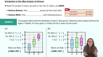
One-Way ANOVA (Analysis of Variance)

One-Way ANOVA is used to compare the means of three or more independent groups to determine if at least one group mean is statistically different. It assumes normality, independence, and equal variances, making it suitable for testing wage differences across the three states.
Recommended video:
06:46
Introduction to ANOVA

Significance Level and Decision Rule

The significance level (α = 0.01) defines the threshold for rejecting the null hypothesis, controlling the probability of a Type I error. After calculating the ANOVA F-statistic and corresponding p-value, if p ≤ α, reject H0; otherwise, fail to reject H0, concluding whether wage differences are statistically significant.
Recommended video:
03:53
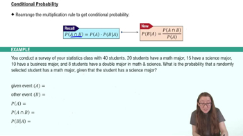
Conditional Probability Rule
Related Practice
Textbook Question

Performing a Chi-Square Goodness-of-Fit Test

In Exercises 7–16, (b) find the critical value and identify the rejection region.


Ways to Pay A financial analyst claims that the distribution of people’s preferences on how to pay for goods is different from the distribution shown in the figure. You randomly select 600 people and record their preferences on how to pay for goods. The table shows the results. At α=0.01, test the financial analyst’s claim. (Adapted from Travis Credit Union)


49
views
Textbook Question

Performing a Chi-Square Goodness-of-Fit Test

In Exercises 7–16, (a) identify the claim and state H₀ and Hₐ.


Ways to Pay A financial analyst claims that the distribution of people’s preferences on how to pay for goods is different from the distribution shown in the figure. You randomly select 600 people and record their preferences on how to pay for goods. The table shows the results. At α=0.01, test the financial analyst’s claim. (Adapted from Travis Credit Union)


71
views
Textbook Question

In each exercise,

e. interpret the decision in the context of the original claim.

[APPLET] In Exercises 1–3, use the data, which list the hourly wages (in dollars) for randomly selected surgical technologists from three states. Assume the wages are normally distributed and that the samples are independent. (Adapted from U.S. Bureau of Labor Statistics)

Maine: 22.76, 27.60, 25.08, 17.01, 30.15, 27.09, 20.95, 25.52, 20.11, 23.67, 24.32

Oklahoma: 24.64, 21.66, 19.38, 18.19, 23.14, 20.58, 19.53, 30.77, 27.46, 23.80

Massachusetts: 27.07, 24.71, 32.80, 28.34, 33.45, 33.36, 36.81, 30.04, 29.01, 24.30, 29.22, 29.50

Are the mean hourly wages of surgical technologists the same for all three states? Use α=0.01. Assume that the population variances are equal.

21
views
Textbook Question

In Exercises 9–12, find the critical F-value for a right-tailed test using the level of significance α and degrees of freedom d.f.N and d.f.D.


α=0.05,d.f.N=20,d.f.D=25

78
views
Textbook Question

In Exercises 1–4, (a) identify the claim and state H₀ and Hₐ, (b) find the critical value and identify the rejection region, (c) find the chi-square test statistic, (d) decide whether to reject or fail to reject the null hypothesis, and (e) interpret the decision in the context of the original claim.


A sports website claims that the opinions of golfers about what irritates them the most on the golf course are distributed as shown in the pie chart. You randomly select 1018 golfers and ask them what irritates them the most on the golf course. The table shows the results. At α=0.05, test the sports website’s claim. (Adapted from GOLF.com)


58
views
Textbook Question

In Exercises 13–16, find the critical F-value for a two-tailed test using the level of significance α and degrees of freedom d.f.N and d.f.D.


α=0.01,d.f.N=40,d.f.D=60

63
views