Frequency Polygons: Videos & Practice Problems

Frequency polygons are an alternative to histograms for displaying frequency distributions, using points connected by segments instead of bars. Both graphs share the same axes, with the y-axis representing frequencies and the x-axis labeled with class midpoints, calculated as the average of class limits. To assess skewness, identify the peak and observe the tails; a left tail indicates left skew, a right tail indicates right skew, and balanced tails suggest no skew. Understanding these concepts enhances data interpretation and visualization skills in statistics.

Creating Frequency Polygons

When displaying data in a frequency distribution, a histogram is often the go-to choice, but a frequency polygon is another effective option. A frequency polygon uses points connected by line segments to represent the same data as a histogram, allowing for a clear visualization of frequencies across different classes.

To create a frequency polygon, start by plotting points for each class based on their frequencies. For instance, if the frequency of the first class is six, you would plot a point at the corresponding x-axis position with a y-coordinate of six. Continue this process for each class, connecting the points with line segments to form the polygon. It’s important to note that the y-axis for both the histogram and frequency polygon displays frequencies, and the x-axis is labeled with class midpoints, which can be calculated by averaging the lower and upper limits of each class.

For example, if the lower limit of a class is 0 and the upper limit is 24, the midpoint is calculated as:

Midpoint = \(\frac{0 + 24}{2} = 12\)

Once all midpoints are determined, label the x-axis accordingly. This allows for easy interpretation of the data; for instance, a point at (12, 6) indicates that there are six individuals in the age range corresponding to that midpoint.

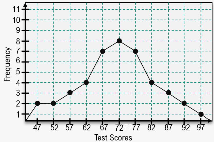
While frequency polygons may resemble line graphs, they serve a different purpose. They do not imply that there are exact counts at specific points but rather represent the frequency of data within defined ranges. Additionally, when assessing skewness in the data, both histograms and frequency polygons are analyzed similarly. The peak of the distribution is identified, and the tails are examined. A left tail indicates left skew, a right tail indicates right skew, and a balanced distribution suggests no skew. For example, if the peak occurs at a midpoint of 37 with a frequency of eight, and the tails are relatively equal, the data can be classified as not skewed.

Understanding how to create and interpret frequency polygons enhances your ability to analyze and present data effectively, providing a valuable tool for visualizing distributions.

Using the frequency polygon below, what range of test scores was most popular? 

• A. 72
• B. 70-74
• C. 70.5-74.5
• D. 67-77

Answer: (B)

Frequency Polygons Example 1

In this example, we explore how to analyze a frequency polygon that represents the age distribution of individuals in a subway car. Understanding how to derive class midpoints, identify popular age groups, and calculate totals within specific age ranges is essential for interpreting frequency data.

To find the class midpoint for the age group 18 to 20, we add the lower limit (18) and the upper limit (20) and divide by two. This calculation is as follows:

Class Midpoint = \(\frac{18 + 20}{2} = \frac{38}{2} = 19\).

Thus, the class midpoint for this age group is 19, which we can label on the x-axis of our frequency polygon. Notably, the class midpoints are evenly spaced, increasing by three for each subsequent age group.

Next, we determine the most and least popular age groups based on frequency. The most popular age group corresponds to the highest frequency observed, which is 8, occurring at the class midpoint of 34. This indicates that the most popular age range is from 33 to 35. Conversely, the least popular age groups are identified by the lowest frequency, which is 1, occurring at two class midpoints: 19 (representing ages 18 to 20) and 50 (representing ages 49 to 51).

Finally, to find the total number of individuals aged between 27 and 35, we identify the relevant age classes. The age group 27 to 29 has a frequency of 4, the group 30 to 32 has a frequency of 7, and the group 33 to 35 has a frequency of 8. By summing these frequencies, we calculate:

Total = 4 (ages 27-29) + 7 (ages 30-32) + 8 (ages 33-35) = 19.

Thus, there are 19 individuals in the subway car aged between 27 and 35.

Here’s what students ask on this topic:

What is a frequency polygon and how is it different from a histogram?

A frequency polygon is a graphical representation of a frequency distribution that uses points connected by straight line segments to display data. It differs from a histogram, which uses bars to represent frequencies. In a frequency polygon, the x-axis is labeled with class midpoints, calculated as the average of the lower and upper limits of each class, while the y-axis represents frequencies. The points are plotted at the class midpoints based on their frequencies and connected to form the polygon. Unlike histograms, frequency polygons provide a smoother visual representation of data trends and are particularly useful for comparing multiple distributions on the same graph.

How do you calculate class midpoints for a frequency polygon?

Class midpoints are calculated by finding the average of the lower and upper limits of a class. The formula for calculating a class midpoint is:

$\mathrm{Midpoint}=\frac{\mathrm{Lower}+\mathrm{Upper}}{2}$

For example, if the lower limit of a class is 0 and the upper limit is 24, the midpoint is:

$\mathrm{Midpoint}=\frac{0+24}{2}=12$

These midpoints are used to label the x-axis in a frequency polygon and help in plotting the points corresponding to the frequencies of each class.

How do you interpret skewness in a frequency polygon?

To interpret skewness in a frequency polygon, start by identifying the peak, which corresponds to the highest frequency. Then, examine the tails on either side of the peak. If the tail extends further to the left, the data is left-skewed. If the tail extends further to the right, the data is right-skewed. If the tails are approximately equal in length, the data is symmetric and has no skew. For example, if the peak occurs at a midpoint of 37 with a frequency of 8, and the tails on both sides are balanced, the data is not skewed. This method is similar to analyzing skewness in histograms, but the visual representation in a frequency polygon makes it easier to observe trends and symmetry.

What are the advantages of using a frequency polygon over a histogram?

Frequency polygons offer several advantages over histograms. First, they provide a smoother visual representation of data trends, making it easier to identify patterns and compare distributions. Second, frequency polygons can display multiple datasets on the same graph, allowing for direct comparison. Third, they require less space and are visually less cluttered, especially when dealing with overlapping data. Additionally, frequency polygons are useful for showing cumulative frequency distributions and are easier to interpret when analyzing skewness or symmetry. While histograms are ideal for discrete data, frequency polygons are better suited for continuous data and comparative analysis.

How do you plot a frequency polygon step by step?

To plot a frequency polygon, follow these steps:

1. Calculate the class midpoints using the formula: $\mathrm{Midpoint}=\frac{\mathrm{Lower}+\mathrm{Upper}}{2}$.
2. Label the x-axis with the class midpoints and the y-axis with frequencies.
3. Plot points at the class midpoints, with the y-coordinate corresponding to the frequency of each class.
4. Connect the points with straight line segments.
5. Extend the first and last points to the x-axis to complete the polygon.

This process creates a frequency polygon that visually represents the distribution of data and allows for easy interpretation of trends and skewness.

Can frequency polygons be used to compare multiple datasets?

Yes, frequency polygons are excellent for comparing multiple datasets. To do this, plot separate frequency polygons for each dataset on the same graph. Use different colors or line styles to distinguish between the datasets. Since frequency polygons use points and lines instead of bars, they allow for overlapping data to be visualized clearly. This makes it easier to compare trends, peaks, and skewness across datasets. For example, you can compare the age distributions of bus riders in two different cities by plotting their frequency polygons on the same axes, enabling direct visual comparison.