How do you determine the number of pairs for the Bonferroni test?

The number of pairs in the Bonferroni test corresponds to the number of unique pairwise comparisons between group means. If you have k groups, the number of pairs is given by the combination formula: C ( k , 2 ) = k ! ( k − 2 ) ! 2 ! This calculates how many unique pairs of groups can be formed. For example, with 3 groups, there are 3 pairs: (1,2), (2,3), and (1,3). This number is used to adjust p-values in the Bonferroni correction.

14. ANOVA

Multiple Comparisons: Bonferoni Test

14. ANOVA

Multiple Comparisons: Bonferoni Test: Videos & Practice Problems

Video Lessons Practice

Topic summary

Post hoc tests, such as the Bonferroni test, identify which means differ after rejecting the null hypothesis in a one-way ANOVA. This involves pairwise comparisons using a t-test formula with the mean square error (MSE) from ANOVA as variance within. Adjusted p-values are calculated by multiplying the original p-value by the number of pairs to control the experiment-wide error rate (alpha). This method ensures accurate identification of significant differences between group means, enhancing inferential statistics and hypothesis testing in analysis of variance (ANOVA).

concept

The Bonferroni Test

Video duration:

The Bonferroni Test Video Summary

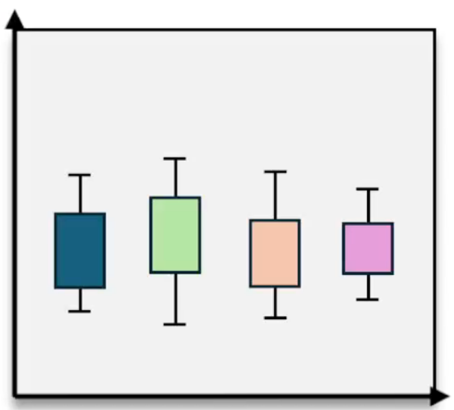
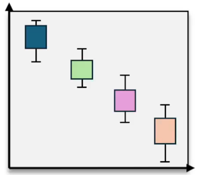
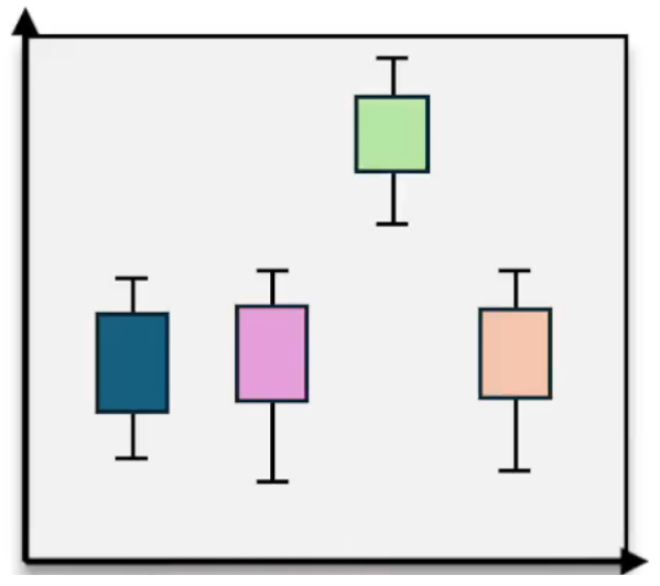
When conducting a one-way ANOVA test, rejecting the null hypothesis indicates that at least one group mean differs from the others. However, this result does not specify which means are different. To identify the specific pairs of means that differ, a follow-up procedure called a post hoc test is used. One common post hoc test is the Bonferroni test, which compares pairs of group means while controlling for the increased risk of Type I error due to multiple comparisons.

The Bonferroni test works by breaking down the multiple group means into all possible pairs and performing individual two-sample t-tests on each pair. For example, if there are three groups (such as grades 10, 11, and 12), the pairs tested would be (10 vs. 11), (11 vs. 12), and (10 vs. 12). Each pair is tested with the null hypothesis that the two means are equal, and the alternative hypothesis that they are not equal, making it a two-tailed test.

Key values needed for the Bonferroni test come from the ANOVA output, including the Mean Square Error (MSE), which represents the variance within groups. This MSE is used as the estimate of variance in the t-test calculations. Other important parameters include the total sample size (N), the number of groups (k), and the degrees of freedom for error, calculated as $df = N - k$.

The test statistic for each pairwise comparison is calculated using the formula:

\[t = \frac{\bar{x}_1 - \bar{x}_2}{\sqrt{MSE \left(\frac{1}{n_1} + \frac{1}{n_2}\right)}}\]

where $\bar{x}_1$ and $\bar{x}_2$ are the sample means of the two groups, $n_1$ and $n_2$ are their respective sample sizes, and $MSE$ is the mean square error from the ANOVA.

After calculating the t-statistic, the corresponding p-value is found using the t-distribution with the appropriate degrees of freedom. Since the test is two-tailed, the p-value is doubled. However, because multiple pairwise tests are conducted, the Bonferroni correction adjusts for the increased chance of false positives by multiplying each p-value by the number of comparisons (pairs). This adjustment ensures the overall Type I error rate remains at the chosen significance level, typically $\alpha = 0.05$.

The number of pairs can be calculated using combinations: for $k$ groups, the number of pairs is given by the binomial coefficient:

\[\binom{k}{2} = \frac{k(k-1)}{2}\]

For example, with three groups, there are three pairs.

Once the adjusted p-values are obtained, each is compared to the significance level $\alpha$. If the adjusted p-value is less than $\alpha$, the null hypothesis for that pair is rejected, indicating a statistically significant difference between those two group means. If the adjusted p-value is greater than $\alpha$, there is insufficient evidence to conclude a difference.

In practice, the Bonferroni test can be tedious due to multiple calculations, but it provides a rigorous method to pinpoint which specific group means differ after an overall ANOVA indicates a difference exists. This approach helps maintain control over Type I error rates while allowing detailed pairwise comparisons.

Study Smarter with Worksheets.

Follow along with each video using our printable worksheets

Problem

A researcher is comparing mean cholesterol levels across 4 diet plans (A, B, C, D) in a One-Way ANOVA test. If $H sub 0$ was rejected and the researcher were to use a Bonferroni Test, how many pairs of comparisons would they do?

$12$

$6$

$4$

$16$

Problem

For which of the following scenarios would it be most appropriate to run a Bonferroni Test to see which mean(s) are significantly different from the rest?

Box plots of four groups with varying medians and ranges, used to compare group differences visually.

Box plots in descending order with error bars showing data spread for multiple group comparisons.

Box plots of four groups with varying medians and ranges, showing data distribution and variability for comparison.

example

The Bonferroni Test Example 1

Video duration:

The Bonferroni Test Example 1 Video Summary

When comparing the taste ratings of three different cereal brands, an initial analysis using ANOVA (Analysis of Variance) can determine if there is a significant difference among the mean ratings. The null hypothesis in ANOVA states that all group means are equal, while rejecting this hypothesis indicates that at least one mean differs. After confirming that the ANOVA null hypothesis is rejected, pairwise comparisons can be conducted to identify which specific groups differ. One common method for these comparisons is the Bonferroni test, which adjusts for multiple comparisons to control the overall Type I error rate.

In this context, the Bonferroni test focuses on comparing the means of cereal A and cereal C. The hypotheses for this two-tailed test are:

$H_0: \mu_A = \mu_C$

$H_a: \mu_A \neq \mu_C$

The test statistic for comparing two means with equal variances is calculated using the formula:

\[t = \frac{\bar{x}_A - \bar{x}_C}{\sqrt{MSE \left(\frac{1}{n_A} + \frac{1}{n_C}\right)}}\]

where $\bar{x}_A$ and $\bar{x}_C$ are the sample means, $MSE$ is the mean square error from the ANOVA output, and $n_A$ and $n_C$ are the sample sizes for groups A and C respectively. The degrees of freedom for this test are calculated as $df = N - k$, where $N$ is the total number of observations and $k$ is the number of groups.

For example, if the sample means are 7.67 for cereal A and 8.0 for cereal C, with an $MSE$ of 0.944 and sample sizes of 6 each, the test statistic is:

\[t = \frac{7.67 - 8.0}{\sqrt{0.944 \left(\frac{1}{6} + \frac{1}{6}\right)}} = -0.588\]

The corresponding p-value is found by calculating the probability of observing a test statistic as extreme as this under the null hypothesis. Using the t-distribution with 15 degrees of freedom, the two-tailed p-value is approximately 0.565. However, because multiple pairwise comparisons are being made, the Bonferroni correction adjusts the p-value by multiplying it by the number of comparisons (in this case, 3):

\[p_{\text{adjusted}} = p \times 3 = 0.565 \times 3 = 1.695\]

Since p-values cannot exceed 1, this is capped at 1. Because the adjusted p-value is much greater than the significance level $\alpha = 0.05$, we fail to reject the null hypothesis, indicating no significant difference between the means of cereals A and C.

In contrast, comparisons between cereals A and B, and cereals B and C, yield very low p-values (e.g., 0.0014 and 0.0004), leading to rejection of the null hypotheses for those pairs. This suggests that cereal B's mean rating is significantly different from both A and C, while A and C are similar. Such pairwise comparisons following ANOVA help pinpoint which specific groups differ, providing clearer insights into the data.

Do you want more practice?

Here’s what students ask on this topic:

The Bonferroni test is a post hoc test used after rejecting the null hypothesis in a one-way ANOVA. Its purpose is to identify which specific group means differ from each other. Since ANOVA only tells us that at least one mean is different, the Bonferroni test performs pairwise comparisons between group means to pinpoint the differences. It adjusts for the increased risk of Type I error that occurs when multiple comparisons are made by multiplying the p-values by the number of pairs tested. This correction controls the overall experiment-wise error rate, ensuring that the conclusions about which means differ are statistically reliable.

To calculate the test statistic for the Bonferroni test, you use a t-score similar to a two-sample t-test. The formula is:

t = x̄

₁−x̄₂MSE(1n₁+1n₂)

Here, $x̄$ ₁ and $x̄$ ₂ are the sample means of the two groups being compared, $MSE$ is the mean square error from the ANOVA, and $n$ ₁ and $n$ ₂ are the sample sizes of the two groups. This t-score is then used to find the p-value for the pairwise comparison.

The Bonferroni correction is a method used to adjust p-values when performing multiple pairwise comparisons to control the overall Type I error rate. When multiple tests are conducted, the chance of incorrectly rejecting at least one true null hypothesis (false positive) increases. The correction involves multiplying each individual p-value by the number of comparisons (pairs) made. Alternatively, the significance level α can be divided by the number of comparisons. This adjustment ensures that the probability of making one or more Type I errors across all tests remains at the desired significance level, typically 0.05, making the results more reliable.

The number of pairs in the Bonferroni test corresponds to the number of unique pairwise comparisons between group means. If you have $k$ groups, the number of pairs is given by the combination formula:

C (k, 2) = \frac{k}{!} (k - 2)! 2!

This calculates how many unique pairs of groups can be formed. For example, with 3 groups, there are 3 pairs: (1,2), (2,3), and (1,3). This number is used to adjust p-values in the Bonferroni correction.

After calculating the adjusted p-values by multiplying the original p-values by the number of pairs, you compare these adjusted p-values to the significance level α (commonly 0.05). If the adjusted p-value for a pair is less than α, you reject the null hypothesis for that pair, concluding that the two group means are significantly different. If the adjusted p-value is greater than α, you fail to reject the null hypothesis, indicating insufficient evidence to say the means differ. This interpretation helps identify which specific groups differ after an overall ANOVA test has shown that at least one difference exists.