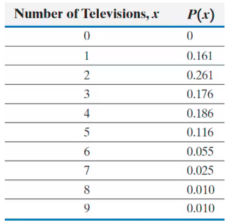
[NW] [DATA] TelevisionsIn the Sullivan Statistics Survey I, individuals were asked to disclose the number of televisions in their household. In the following probability distribution, the random variable X represents the number of televisions in households. a. Confirm that this represents a discrete probability distribution.
Verified step by step guidance
1
Step 1: Verify that the random variable X is discrete by checking if it takes on countable values. Here, X represents the number of televisions, which are whole numbers from 0 to 9, so X is discrete.
Step 2: Check that each probability value P(x) is between 0 and 1 inclusive. Review the given probabilities: 0, 0.161, 0.261, 0.176, 0.186, 0.116, 0.055, 0.025, 0.010, and 0.010. All these values satisfy 0 \(\leq\) P(x) \(\leq\) 1.
Step 3: Confirm that the sum of all probabilities equals 1. Calculate the sum using the formula: \(\sum_{x=0}^{9} P(x) = 0 + 0.161 + 0.261 + 0.176 + 0.186 + 0.116 + 0.055 + 0.025 + 0.010 + 0.010\).
Step 4: If the sum from Step 3 equals 1, then the set of probabilities forms a valid probability distribution for the discrete random variable X.
Step 5: Conclude that since X is discrete, all probabilities are between 0 and 1, and their sum is 1, this table represents a discrete probability distribution.
Verified video answer for a similar problem:
This video solution was recommended by our tutors as helpful for the problem above
Video duration:
2m
Play a video:
0 Comments
Key Concepts
Here are the essential concepts you must grasp in order to answer the question correctly.
Discrete Probability Distribution
A discrete probability distribution lists all possible values of a discrete random variable and their associated probabilities. Each probability must be between 0 and 1, and the sum of all probabilities must equal 1. This ensures the distribution accurately represents the likelihood of each outcome.
Variance & Standard Deviation of Discrete Random Variables
Random Variable
A random variable is a numerical outcome of a random phenomenon. In this case, X represents the number of televisions in a household, which can only take integer values. Understanding the random variable helps in interpreting the probability distribution and analyzing the data.
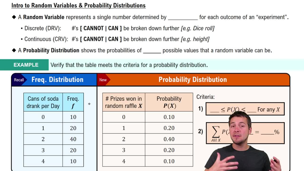
Intro to Random Variables & Probability Distributions
Probability Sum Rule
The probability sum rule states that the total probability of all possible outcomes must be exactly 1. This rule is essential to confirm that a given set of probabilities forms a valid probability distribution, ensuring that all possible events are accounted for.

 Verified step by step guidance
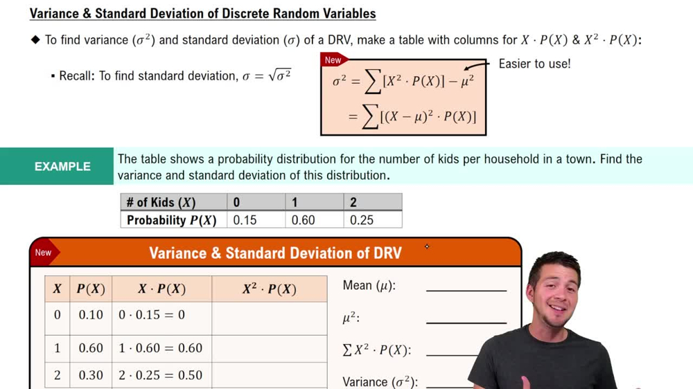
 04:48
04:48