
Ch. 6 - Normal Probability Distributions
Triola - Elementary Statistics 14th Edition
Triola14th EditionElementary StatisticsISBN: 9780137366446Not the one you use?Change textbook
Chapter 6, Problem 6.3.15

Births: Sampling Distribution of Sample Proportion When two births are randomly selected, the sample space for genders is bb, bg, gb, and gg (where and Assume that those four outcomes are equally likely. Construct a table that describes the sampling distribution of the sample proportion of girls from two births. Does the mean of the sample proportions equal the proportion of girls in two births? Does the result suggest that a sample proportion is an unbiased estimator of a population proportion?

Verified step by step guidance
1
Step 1: Understand the problem. The goal is to construct a sampling distribution for the sample proportion of girls from two births. The sample space consists of four equally likely outcomes: bb (both boys), bg (boy and girl), gb (girl and boy), and gg (both girls). Each outcome has a probability of 1/4.
Step 2: Define the sample proportion of girls for each outcome. For each outcome in the sample space, calculate the proportion of girls: bb = 0/2 = 0, bg = 1/2 = 0.5, gb = 1/2 = 0.5, gg = 2/2 = 1.
Step 3: Construct the sampling distribution table. Create a table with two columns: one for the sample proportion of girls and another for the probability of each proportion. The table will look like this: Proportion of Girls (P) = {0, 0.5, 1}, Probability = {1/4, 2/4, 1/4}. Note that the proportion 0.5 occurs twice (bg and gb), so its probability is 2/4.
Step 4: Calculate the mean of the sample proportions. Use the formula for the mean of a probability distribution: \( \mu_P = \sum (P_i \cdot P(P_i)) \), where \( P_i \) is the sample proportion and \( P(P_i) \) is its probability. Substitute the values from the table to compute the mean.
Step 5: Compare the mean of the sample proportions to the population proportion of girls. The population proportion of girls is 0.5 (since there are two equally likely genders). If the mean of the sample proportions equals the population proportion, it suggests that the sample proportion is an unbiased estimator of the population proportion.

Verified video answer for a similar problem:

This video solution was recommended by our tutors as helpful for the problem above.
Video duration:
6m
Was this helpful?

Key Concepts

Here are the essential concepts you must grasp in order to answer the question correctly.

Sampling Distribution

The sampling distribution of a statistic is the probability distribution of that statistic based on a random sample. In this context, it refers to the distribution of the sample proportion of girls from two births. Understanding this concept is crucial for analyzing how sample proportions can vary and how they relate to the true population proportion.
Recommended video:
05:11
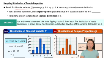
Sampling Distribution of Sample Proportion

Sample Proportion

The sample proportion is the ratio of the number of successes (in this case, the number of girls born) to the total number of trials (the total births in the sample). It is a key statistic used to estimate the population proportion. In this scenario, calculating the sample proportion helps determine the likelihood of observing a certain number of girls in two births.
Recommended video:
05:11
Sampling Distribution of Sample Proportion

Unbiased Estimator

An unbiased estimator is a statistic that, on average, equals the parameter it estimates. In this case, if the mean of the sample proportions equals the true proportion of girls in the population, the sample proportion is considered an unbiased estimator. This concept is essential for evaluating the reliability of sample statistics in estimating population parameters.
Recommended video:
06:33
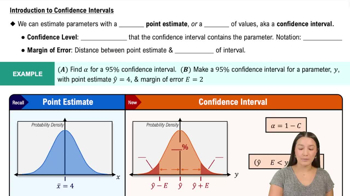
Introduction to Confidence Intervals
Related Practice
Textbook Question

Hypothesis Testing. In Exercises 17–19, apply the central limit theorem to test the given claim. (Hint: See Example 3.)


Adult Sleep Times (hours) of sleep for randomly selected adult subjects included in the National Health and Nutrition Examination Study are listed below. Here are the statistics for this sample: n = 12, x_bar = 6.8 hours, s = 20 hours. The times appear to be from a normally distributed population. A common recommendation is that adults should sleep between 7 hours and 9 hours each night. Assuming that the mean sleep time is 7 hours, find the probability of getting a sample of 12 adults with a mean of 6.8 hours or less. What does the result suggest about a claim that “the mean sleep time is less than 7 hours”?


4 8 4 4 8 6 9 7 7 10 7 8

169
views
Textbook Question

Standard Normal Distribution. In Exercises 9–12, find the area of the shaded region. The graph depicts the standard normal distribution of bone density scores with mean 0 and standard deviation 1.


432
views
Textbook Question

Continuous Uniform Distribution. In Exercises 5–8, refer to the continuous uniform distribution depicted in Figure 6-2 and described in Example 1. Assume that a passenger is randomly selected, and find the probability that the waiting time is within the given range.

Less than 4.00 minutes

227
views
Textbook Question

Distributions In a continuous uniform distribution,


" style="" width="290">


a. Find the mean and standard deviation for the distribution of the waiting times represented in Figure 6-2, which accompanies Exercises 5–8.

246
views
Textbook Question

Standard Normal Distribution. In Exercises 17–36, assume that a randomly selected subject is given a bone density test. Those test scores are normally distributed with a mean of 0 and a standard deviation of 1. In each case, draw a graph, then find the probability of the given bone density test scores. If using technology instead of Table A-2, round answers to four decimal places.


Between 1.50 and 2.00

185
views
Textbook Question

Constructing Normal Quantile Plots. In Exercises 17–20, use the given data values to identify the corresponding z scores that are used for a normal quantile plot, then identify the coordinates of each point in the normal quantile plot. Construct the normal quantile plot, then determine whether the data appear to be from a population with a normal distribution.


Earthquake Depths A sample of depths (km) of earthquakes is obtained from Data Set 24 “Earthquakes” in Appendix B: 17.3, 7.0, 7.0, 7.0, 8.1, 6.8.

139
views