
Textbook Question
In a binomial experiment with n trials and probability of success p, if __ ________, the binomial random variable X is approximately normal with μX = ________ and σX = ________.
77
views
 Verified step by step guidanceVerified video answer for a similar problem:
 04:48
04:48 08:50
08:50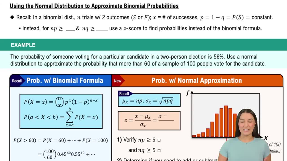 06:23
06:23