"In Problems 5–14, a discrete random variable is given. Assume the probability of the random variable will be approximated using the normal distribution. Describe the area under the normal curve that will be computed. For example, if we wish to compute the probability of finding at least five defective items in a shipment, we would approximate the probability by computing the area under the normal curve to the right of x = 4.5. The probability that more than 20 people want to see the marriage tax penalty abolished"
Verified step by step guidance
1
Identify the discrete random variable and the event of interest. Here, the event is "more than 20 people want to see the marriage tax penalty abolished," which corresponds to the random variable X being greater than 20, i.e., X > 20.
Since the problem involves approximating a discrete distribution with a normal distribution, apply the continuity correction. For the event X > 20, this means we approximate P(X > 20) by P(X > 20.5) in the continuous normal distribution.
Determine the mean (\$\(\mu\)\$) and standard deviation (\$\(\sigma\)\$) of the original discrete random variable. These parameters are necessary to define the corresponding normal distribution used for approximation.
Translate the corrected value (20.5) into a z-score using the formula:
\[z = \frac{20.5 - \mu}{\sigma}\]
This standardizes the value to the standard normal distribution.
The probability that more than 20 people want to see the marriage tax penalty abolished is approximated by the area under the normal curve to the right of z, i.e., P(Z > z). This corresponds to the area under the normal curve for values greater than 20.5 in the original scale.
Verified video answer for a similar problem:
This video solution was recommended by our tutors as helpful for the problem above
Video duration:
4m
Play a video:
0 Comments
Key Concepts
Here are the essential concepts you must grasp in order to answer the question correctly.
Discrete to Continuous Approximation
When a discrete random variable is approximated by a continuous distribution like the normal, a continuity correction is applied. This involves adjusting the discrete value by 0.5 to better estimate probabilities, such as using x = 20.5 instead of 20 when calculating areas under the normal curve.
Variance & Standard Deviation of Discrete Random Variables
Normal Distribution and Area Under the Curve
The normal distribution is a continuous, symmetric bell-shaped curve used to approximate probabilities. The probability of an event corresponds to the area under the curve over a specific interval, which can be found using z-scores and standard normal tables or software.
To find probabilities like 'more than 20,' we interpret this as P(X > 20). Using the continuity correction, this becomes P(X > 20.5) for the normal approximation, meaning we calculate the area under the normal curve to the right of 20.5.

 Verified step by step guidance
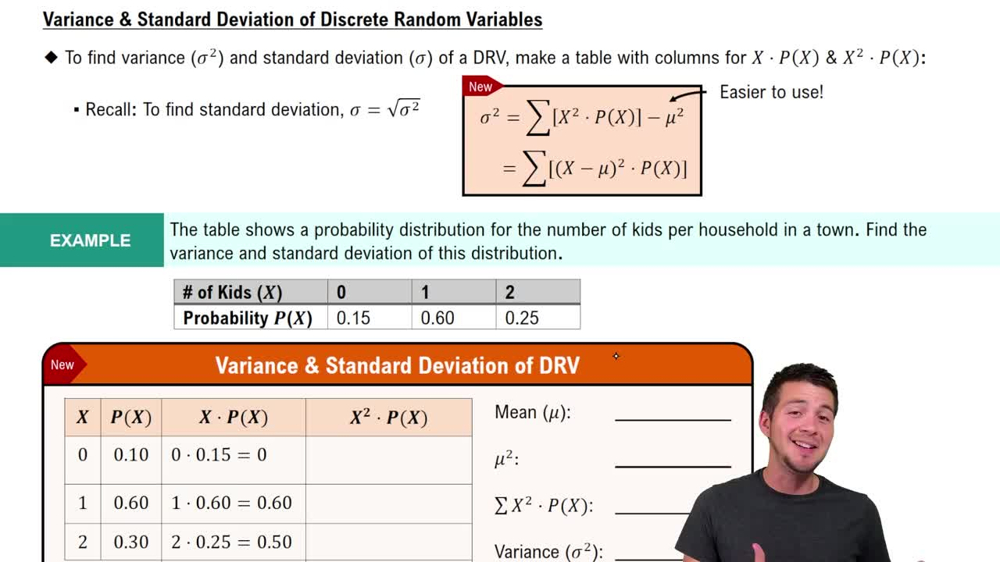
 04:48
04:48