Suppose the scores earned on Professor McArthur’s third statistics exam are normally distributed with mean 64 and standard deviation 8. Professor McArthur wants to curve the exam scores as follows: The top 6% get an A, the next 14% get a B, the middle 60% get a C, the bottom 6% fail, and the rest earn a D. Any student who can determine these cut-offs earns five bonus points. Determine the cut-offs for Professor McArthur.
Table of contents
- 1. Intro to Stats and Collecting Data1h 14m
- 2. Describing Data with Tables and Graphs1h 56m
- 3. Describing Data Numerically2h 0m
- 4. Probability2h 17m
- 5. Binomial Distribution & Discrete Random Variables3h 6m
- 6. Normal Distribution and Continuous Random Variables2h 11m
- 7. Sampling Distributions & Confidence Intervals: Mean3h 23m
- Sampling Distribution of the Sample Mean and Central Limit Theorem19m
- Distribution of Sample Mean - ExcelBonus23m
- Introduction to Confidence Intervals15m
- Confidence Intervals for Population Mean1h 18m
- Determining the Minimum Sample Size Required12m
- Finding Probabilities and T Critical Values - ExcelBonus28m
- Confidence Intervals for Population Means - ExcelBonus25m
- 8. Sampling Distributions & Confidence Intervals: Proportion2h 10m
- 9. Hypothesis Testing for One Sample5h 8m
- Steps in Hypothesis Testing1h 6m
- Performing Hypothesis Tests: Means1h 4m
- Hypothesis Testing: Means - ExcelBonus42m
- Performing Hypothesis Tests: Proportions37m
- Hypothesis Testing: Proportions - ExcelBonus27m
- Performing Hypothesis Tests: Variance12m
- Critical Values and Rejection Regions28m
- Link Between Confidence Intervals and Hypothesis Testing12m
- Type I & Type II Errors16m
- 10. Hypothesis Testing for Two Samples5h 37m
- Two Proportions1h 13m
- Two Proportions Hypothesis Test - ExcelBonus28m
- Two Means - Unknown, Unequal Variance1h 3m
- Two Means - Unknown Variances Hypothesis Test - ExcelBonus12m
- Two Means - Unknown, Equal Variance15m
- Two Means - Unknown, Equal Variances Hypothesis Test - ExcelBonus9m
- Two Means - Known Variance12m
- Two Means - Sigma Known Hypothesis Test - ExcelBonus21m
- Two Means - Matched Pairs (Dependent Samples)42m
- Matched Pairs Hypothesis Test - ExcelBonus12m
- Two Variances and F Distribution29m
- Two Variances - Graphing CalculatorBonus16m
- 11. Correlation1h 24m
- 12. Regression3h 33m
- Linear Regression & Least Squares Method26m
- Residuals12m
- Coefficient of Determination12m
- Regression Line Equation and Coefficient of Determination - ExcelBonus8m
- Finding Residuals and Creating Residual Plots - ExcelBonus11m
- Inferences for Slope31m
- Enabling Data Analysis ToolpakBonus1m
- Regression Readout of the Data Analysis Toolpak - ExcelBonus21m
- Prediction Intervals13m
- Prediction Intervals - ExcelBonus19m
- Multiple Regression - ExcelBonus29m
- Quadratic Regression15m
- Quadratic Regression - ExcelBonus10m
- 13. Chi-Square Tests & Goodness of Fit2h 21m
- 14. ANOVA2h 29m
6. Normal Distribution and Continuous Random Variables
Non-Standard Normal Distribution
Problem 7.4.5
Textbook Question
"In Problems 5–14, a discrete random variable is given. Assume the probability of the random variable will be approximated using the normal distribution. Describe the area under the normal curve that will be computed. For example, if we wish to compute the probability of finding at least five defective items in a shipment, we would approximate the probability by computing the area under the normal curve to the right of x = 4.5.
The probability that at least 40 households have a gas stove"
 Verified step by step guidance
1
Identify the discrete random variable and the event of interest. Here, the event is "at least 40 households have a gas stove," which means \( X \geq 40 \) where \( X \) is the number of households with a gas stove.
Since \( X \) is discrete, apply the continuity correction to approximate the probability using the normal distribution. For "at least 40," this means considering \( X \geq 39.5 \) in the continuous normal approximation.
Determine the mean \( \mu \) and standard deviation \( \sigma \) of the discrete random variable \( X \). These parameters are necessary to define the corresponding normal distribution \( N(\mu, \sigma^2) \).
Translate the problem into finding the area under the normal curve to the right of \( x = 39.5 \). This corresponds to \( P(X \geq 40) \approx P(Y \geq 39.5) \) where \( Y \sim N(\mu, \sigma^2) \).
Express the probability in terms of the standard normal variable \( Z \) by standardizing: \( Z = \frac{39.5 - \mu}{\sigma} \). Then, the probability is \( P(Z \geq \frac{39.5 - \mu}{\sigma}) \), which is the area under the standard normal curve to the right of this \( Z \)-value.
 Verified video answer for a similar problem:
This video solution was recommended by our tutors as helpful for the problem above
Video duration:
2mPlay a video:
0 Comments
Key Concepts
Here are the essential concepts you must grasp in order to answer the question correctly.
Discrete to Continuous Approximation
This concept involves approximating a discrete probability distribution, like the binomial or Poisson, with a continuous distribution such as the normal distribution. It is useful when the sample size is large, allowing easier calculation of probabilities using the normal curve instead of summing discrete probabilities.
Recommended video:
Guided course

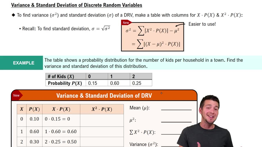
Variance & Standard Deviation of Discrete Random Variables
Continuity Correction
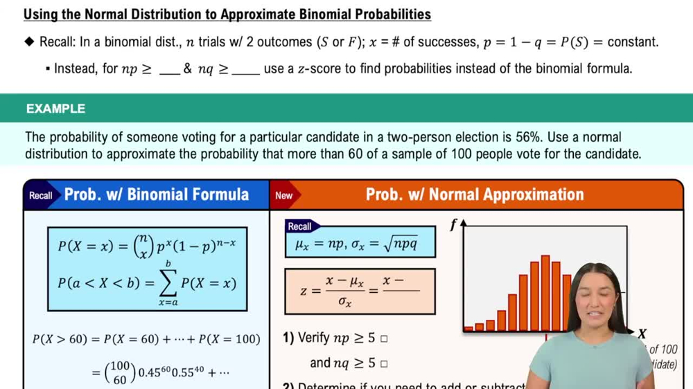
When approximating a discrete distribution with a normal distribution, a continuity correction adjusts for the difference between discrete points and continuous intervals. For example, to find P(X ≥ 40), we calculate the area to the right of 39.5 under the normal curve, improving the accuracy of the approximation.
Recommended video:

Using the Normal Distribution to Approximate Binomial Probabilities
Area Under the Normal Curve
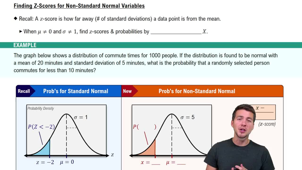
The area under the normal curve represents probabilities for continuous random variables. To find the probability of an event, we calculate the area corresponding to the event's range on the curve, using z-scores and standard normal tables or software to determine the exact probability.
Recommended video:
Guided course

Finding Z-Scores for Non-Standard Normal Variables
Related Videos
Related Practice
Textbook Question
45
views


