Game Boss In video games, a game boss is a powerful non-player...

Question

Game Boss In video games, a game boss is a powerful non-player character created by game developers as an opponent to players of the game. Suppose a game is set up where a player must defeat three bosses and the probability of defeating any boss is 0.20. Assuming each boss battle is independent, the probability distribution for the number of bosses defeated by a player is as follows:

Table showing probabilities of defeating 0 to 3 game bosses: 0–0.512, 1–0.384, 2–0.096, 3–0.008.

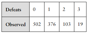
Suppose the game is played by a random sample of 1000 players with the number of bosses defeated recorded. The results are shown below.

Table showing observed counts of players defeating 0 to 3 game bosses: 502, 376, 103, and 19 respectively.

a. Does the distribution of defeats follow the distribution expected by the programmers? Use the alpha = 0.05 level of significance.

Accepted Answer

Welcome back everyone. In this problem, a university registrar wants to understand student enrollment patterns. Suppose a survey is set up where a student chooses between three different online course formats A, B, or C. Assuming each student's choice is independent, the expected probability distribution for the chosen format is as follows. And it's shown in the table below. Suppose the registrar collects data from a random sample of 500 students and the number of students who choose each format is recorded. The results are shown also in the table below. Does the observed distribution of student choices follow the distribution expected by the registrar? Use the significance level alpha of 0.01. A says yes and B says no. Now this problem requires performing a chi square goodness of fit test to determine if the observed distribution of student choices matches the expected probability distribution. So let's state our hypotheses, calculate the expected cones, and compare them to the observed cones to help us figure out if the the observations follow the distribution expected by the registrar. No, for starters. Let's let our null hypothesis OK be that the observed distribution. Our students OK. The observed distribution of students follows the expected probability distribution. OK. Expected probability. Oops, let me write it below here. OK. And that is the distribution that A will have 40% of the sample, uh B will have 35%, and C will have 25%, OK? And if that's the null hypothesis, then the alternate hypothesis must be then that the observed distribution of students. And the observed distribution of students. Does note does not follow. They expected. Probability distribution. Now if this is our null and our alternate hypotheses, then from here we can set our decision rule and basically using the critical value method or decision rule. Would basically say that if our calculated chi squared value. OK. Is greater than our critical chi squared value then we reject our null hypothesis otherwise. If that's not true, in other words, if the critical value is greater than the calculated value, then we fail to reject the null hypothesis. So in this case, we'll need to figure out our we'll need to calculate the chi squared value, uh, find a critical chi squared value from our chi square table, and then compare both. So let's start by calculating our chi squared value using the chi square test statistic, OK? Now, if we recall. The chi-square test statistic basically says our chi squared value is equal to the sum of observed values, OK, minus expected values. OK, squared. Probably I made my, uh my, my, my, my parenthesis too big here. Let me make that a bit smaller. So it's the sum of our observed minus expected values divided by the expected values. So what this means then is that we're going to have a have to set up a table. OK, first we'll have our format there. We'll have our observed values. Our expected values, OK, which is e and of course our observed values would be O and then to make it simpler we can create a column for observed minus expected values, square those, OK, and then divide or squared residual or squared difference bye. So here, let's put all of our formats in our table. So let me, let me come down a bit here, OK? And for our formats. OK, we have, we know, we just finish our columns here. For the formats we know that we have them as A, B, and C, and for a our observed values are 190. B, it's 185, and C, it's 125. Now what about the expected values? What if we go back to our table, remember that we said for A for starters, our expected value would be 40%. Of whatever our sample size would be, that's our expected probability distribution. So since there are 500 students, OK, so for example, since N equals 500. Then the expected value for a, for example, is going to be equal to 40% or 0.4% multiplied by 500, and that would be equal to 200. So for A, the expected value is 200, for B, since the distribution is 0.35, then that would be 35% of 500, which is 175. And for C, since it's 0.25%, then the expected would be 0.25 multiplied by 500, which is 125. So we have all of those values. No, we can compute because our observed minus expected value for A would be 190 minus 200, which is negative 10. When we square that it would be 100, and when we divide that by our expected value that so that's 100 divided by 200, which equals 0.50. Applying the same logic for B their difference will be 10 squared, that's 100. And when we divide that square by E, then we'll get approximately 0.5714. For C, 125 minus 125 is 0, so their square is 0, and thus, the chi square statistic would also be zero. So now if we go ahead and sum here, OK? For starters, we know for observed value, uh, our sum is 500. The expected value of the sum is 500, and if we move on to our chi square test statistic, the sum would be approximately 1.0714. OK? So this is our calculated chi square statistic, test statistic. Now that we have the calculated value, we need to compare it to the critical value. No, From The chi square table, OK, from the chi square table. Where our degrees of freedom equals N1 or K minus 1, the number of categories minus 1, that's 3 minus 1 which equals 2, and a significance level alpha of 0.01, OK. Then our critical chisquared value. Is going to be equal to 9.210. So now that we have our calculated value earlier found as 1.0714, and our critical value of 9.210, what do you notice? Well, when we compare them. Notice that Our calculated value, OK. Our calculated value of 1.0714 is less. OK, than our critical chi squared value of 9.210. And since it's less, that means based on our decision rule, we fail to reject the null hypothesis. So at the 0.01 level of significance there is insufficient evidence to conclude that the observed distribution of student choices for the online course formats differs significantly from the registrar's expected distribution. Therefore, A is the correct answer. Thanks a lot for watching everyone. I hope this video helped.

Key Concepts

Binomial Probability Distribution

Chi-Square Goodness-of-Fit Test

Significance Level and Hypothesis Testing

Watch next