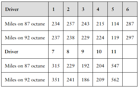
Which of the following is an example of a dependent sample suitable for analysis with the -test?
Table of contents
- 1. Intro to Stats and Collecting Data1h 14m
- 2. Describing Data with Tables and Graphs1h 55m
- 3. Describing Data Numerically2h 5m
- 4. Probability2h 16m
- 5. Binomial Distribution & Discrete Random Variables3h 6m
- 6. Normal Distribution and Continuous Random Variables2h 11m
- 7. Sampling Distributions & Confidence Intervals: Mean3h 23m
- Sampling Distribution of the Sample Mean and Central Limit Theorem19m
- Distribution of Sample Mean - Excel23m
- Introduction to Confidence Intervals15m
- Confidence Intervals for Population Mean1h 18m
- Determining the Minimum Sample Size Required12m
- Finding Probabilities and T Critical Values - Excel28m
- Confidence Intervals for Population Means - Excel25m
- 8. Sampling Distributions & Confidence Intervals: Proportion1h 25m
- 9. Hypothesis Testing for One Sample3h 29m
- 10. Hypothesis Testing for Two Samples4h 50m
- Two Proportions1h 13m
- Two Proportions Hypothesis Test - Excel28m
- Two Means - Unknown, Unequal Variance1h 3m
- Two Means - Unknown Variances Hypothesis Test - Excel12m
- Two Means - Unknown, Equal Variance15m
- Two Means - Unknown, Equal Variances Hypothesis Test - Excel9m
- Two Means - Known Variance12m
- Two Means - Sigma Known Hypothesis Test - Excel21m
- Two Means - Matched Pairs (Dependent Samples)42m
- Matched Pairs Hypothesis Test - Excel12m
- 11. Correlation1h 24m
- 12. Regression1h 50m
- 13. Chi-Square Tests & Goodness of Fit2h 21m
- 14. ANOVA1h 57m
10. Hypothesis Testing for Two Samples
Two Means - Matched Pairs (Dependent Samples)
Problem 11.2.18d
Textbook Question
"[DATA] Does Octane Matter? Octane is a measure of how much fuel can be compressed before it spontaneously ignites. Some people believe that higher-octane fuels result in better gas mileage for their cars. To test this claim, a researcher randomly selected 11 individuals (and their cars) to participate in the study. Each participant received 10 gallons of gas and drove his or her car on a closed course that simulated both city and highway driving. The number of miles driven until the car ran out of gas was recorded. A coin flip was used to determine whether the car was filled up with 87-octane or 92-octane fuel first, and the driver did not know which type of fuel was in the tank. The results are in the following table:

d. The differences are computed as “92 octane minus 87 octane.” The normal probability plot of the differences is shown in the next column. The correlation between the differenced data and the expected z-scores is 0.966. Is there reason to believe that the differences are normally distributed? Conclude that the differences can be normally distributed even though the original data are not.

Verified step by step guidance1
Step 1: Understand the context and data. The problem involves paired data where each driver’s car is tested with two types of fuel (87 octane and 92 octane). The differences are calculated as '92 octane miles minus 87 octane miles' for each driver.
Step 2: Recognize the purpose of the normal probability plot. This plot is used to assess whether the differences follow a normal distribution by comparing the ordered differences to the expected z-scores from a normal distribution.
Step 3: Interpret the correlation value. The correlation between the differenced data and the expected z-scores is 0.966, which is very close to 1. This high correlation suggests that the differences closely follow a straight line on the normal probability plot, indicating approximate normality.
Step 4: Use the normal probability plot visual. The plot shows points that lie roughly along a straight line without large deviations or systematic patterns, reinforcing the conclusion that the differences can be considered normally distributed.
Step 5: Conclude based on the evidence. Even if the original data (miles driven on each fuel type separately) are not normally distributed, the differences between paired observations can be normally distributed. This justifies using statistical methods that assume normality of the differences.
Verified video answer for a similar problem:This video solution was recommended by our tutors as helpful for the problem above
Video duration:
2mPlay a video:
Was this helpful?
Key Concepts
Here are the essential concepts you must grasp in order to answer the question correctly.
Paired Differences
Paired differences involve comparing two related measurements from the same subject or entity, such as miles driven on 92-octane versus 87-octane fuel for the same driver. This approach controls for individual variability, allowing a more precise assessment of the effect of the treatment or condition.
Recommended video:
Guided course
Introduction to Matched Pairs
Normality Assumption in Paired Differences
Many statistical tests, like the paired t-test, assume that the differences between paired observations are approximately normally distributed. This assumption can be checked using a normal probability plot, where data points closely following a straight line indicate approximate normality.
Recommended video:
Guided course
Matched Pairs: Hypothesis Tests
Correlation in Normal Probability Plot
The correlation between ordered differences and expected z-scores in a normal probability plot quantifies how well the data fit a normal distribution. A high correlation (close to 1) suggests the differences are normally distributed, justifying the use of parametric tests even if the original data are not normal.
Recommended video:
Guided course
Correlation Coefficient
Watch next
Master Introduction to Matched Pairs with a bite sized video explanation from Patrick
Start learningRelated Videos
Related Practice
Multiple Choice
15
views
