Textbook Question
"Finding a Critical F-Value for a Right-Tailed Test In Exercises 5–8, find the critical F-value for a right-tailed test using the level of significance α and degrees of freedom d.f.N and d.f.D.
α=0.025, d.f.N=7, d.f.D=3"
70
views

 Verified step by step guidance
 08:24
08:24 05:52
05:52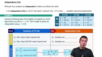 06:28
06:28"Finding a Critical F-Value for a Right-Tailed Test In Exercises 5–8, find the critical F-value for a right-tailed test using the level of significance α and degrees of freedom d.f.N and d.f.D.
α=0.025, d.f.N=7, d.f.D=3"
Finding Expected Frequencies
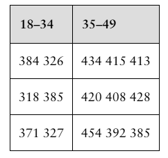
In Exercises 7–12, (a) calculate the marginal frequencies and (b) find the expected frequency for each cell in the contingency table. Assume that the variables are independent.
Performing a Two-Sample F-Test In Exercises 19–26, (a) identify the claim and state H0 and Ha, (b) find the critical value and identify the rejection region, (c) find the test statistic F, (d) decide whether to reject or fail to reject the null hypothesis, and (e) interpret the decision in the context of the original claim. Assume the samples are random and independent, and the populations are normally distributed.
Annual Salaries An employment information service claims that the standard deviation of the annual salaries for public relations managers is less in Louisiana than in Florida. You select a sample of public relations managers from each state. The results of each survey are shown in the figure. At α=0.05, can you support the service’s claim? (Adapted from America’s Career InfoNet)
"In Exercises 13–18, test the claim about the difference between two population variances σ₁² and σ₂² at the level of significance α. Assume the samples are random and independent, and the populations are normally distributed.
Claim: σ₁² = σ₂²; α = 0.05.
Sample statistics: s₁² = 310, n₁ = 7 and s₂² = 297, n₂ = 8"
Testing for Normality Using a chi-square goodness-of-fit test, you can decide, with some degree of certainty, whether a variable is normally distributed. In all chi-square tests for normality, the null and alternative hypotheses are as listed below.
H₀: The variable has a normal distribution.
Hₐ: The variable does not have a normal distribution.
To determine the expected frequencies when performing a chi-square test for normality, first estimate the mean and standard deviation of the frequency distribution. Then, use the mean and standard deviation to compute the z-score for each class boundary. Then, use the z-scores to calculate the area under the standard normal curve for each class. Multiplying the resulting class areas by the sample size yields the expected frequency for each class.In Exercises 17 and 18, (a) find the expected frequencies, (b) find the critical value and identify the rejection region, (c) find the chi-square test statistic, (d) decide whether to reject or fail to reject the null hypothesis, and (e) interpret the decision in the context of the original claim.
In Exercises 17 and 18, (a) find the expected frequencies, (b) find the critical value and identify the rejection region, (c) find the chi-square test statistic, (d) decide whether to reject or fail to reject the null hypothesis, and (e) interpret the decision in the context of the original claim.
Test Scores At α=0.05, test the claim that the 400 test scores shown in the frequency distribution are normally distributed.
Performing a Chi-Square Independence Test In Exercises 13–28, perform the indicated chi-square independence test by performing the steps below.
a. Identify the claim and state H₀ and Hₐ
b. Determine the degrees of freedom, find the critical value, and identify the rejection region.
c. Find the chi-square test statistic.
d. Decide whether to reject or fail to reject the null hypothesis.
e. Interpret the decision in the context of the original claim.
Choosing a College The contingency table shows the results of a survey asking 1858 parents and students of different incomes what their deciding factor was in choosing a college. At α=0.01, can you conclude that the deciding factor in choosing a college is related to the income of the family? (Adapted from Sallie Mae)