Testing for a Linear Correlation
In Exercises 13–28, construct a scatterplot, and find the value of the linear correlation coefficient r. Also find the P-value or the critical values of r from Table A-6. Use a significance level of α = 0.05. Determine whether there is sufficient evidence to support a claim of a linear correlation between the two variables. (Save your work because the same data sets will be used in Section 10-2 exercises.)
Taxis Using the data from Exercise 15, is there sufficient evidence to support the claim that there is a linear correlation between the distance of the ride and the fare (cost of the ride)?

Verified step by step guidance

1. Step 1: Begin by plotting a scatterplot of the data. Plot the distance of the ride on the x-axis and the fare (cost of the ride) on the y-axis. This will help visualize whether there appears to be a linear relationship between the two variables.
2. Step 2: Calculate the linear correlation coefficient (r) using the formula: r = (Σ((x - x̄)(y - ȳ))) / √(Σ(x - x̄)² * Σ(y - ȳ)²). Here, x̄ and ȳ are the means of the x and y variables, respectively. This coefficient measures the strength and direction of the linear relationship.
3. Step 3: Determine the critical values of r or the P-value. Use Table A-6 (or a statistical software) to find the critical values of r for the given sample size and significance level α = 0.05. Alternatively, calculate the P-value associated with the computed r.
4. Step 4: Compare the absolute value of the calculated r to the critical value (or compare the P-value to α). If |r| > critical value or if P-value < α, there is sufficient evidence to support the claim of a linear correlation.
5. Step 5: Conclude whether there is sufficient evidence to support the claim of a linear correlation between the distance of the ride and the fare. If the evidence supports the claim, state that a linear correlation exists; otherwise, state that there is no sufficient evidence for a linear correlation.

Key Concepts

Linear Correlation Coefficient (r)

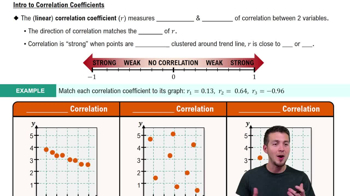
The linear correlation coefficient, denoted as r, quantifies the strength and direction of a linear relationship between two variables. Its value ranges from -1 to 1, where 1 indicates a perfect positive correlation, -1 indicates a perfect negative correlation, and 0 suggests no linear correlation. Understanding r is crucial for assessing how closely the data points cluster around a straight line in a scatterplot.

P-value

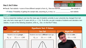
The P-value is a statistical measure that helps determine the significance of results obtained in hypothesis testing. It represents the probability of observing the data, or something more extreme, assuming the null hypothesis is true. A P-value less than the significance level (α = 0.05 in this case) indicates strong evidence against the null hypothesis, suggesting that a linear correlation may exist between the variables.

Scatterplot

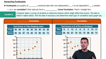
A scatterplot is a graphical representation of two quantitative variables, where each point represents an observation. It helps visualize the relationship between the variables, allowing for the identification of patterns, trends, or correlations. Constructing a scatterplot is a fundamental step in analyzing data, as it provides an intuitive understanding of how the variables interact before calculating statistical measures like the correlation coefficient.